This post is about our paper Causal Bandits without Graph Learning, refer to the full paper for more information.
What are Causal Bandits?
Stochastic bandits are commonly studied problems aimed at modeling online decision making processes. In stochastic multi-armed bandits an agent selects which of $K$ arms to pull in each of $T$ rounds. After each pull the agent receives stochastic reward $R_t$ coming from distribution $\mathbb{P}_{A_t}(\cdot)$ assuming that $A_t$ denotes the arm pulled at the beginning of the round $t$. In this setting a common goal is to maximize the total expected reward received during the $T$ rounds of interaction, or equivalently to minimize the regret. Denote with $\mu_a$ the expected reward of pulling arm $a\in[K]$, where $[K]={\{1,\dots,K}\}$, then the cumulative regret is defined to be:
\begin{equation}
Reg_T=T\max_{a\in[K]}\mu_a-\sum_{t=1}^T\mathbb{E}[R_t].
\end{equation}

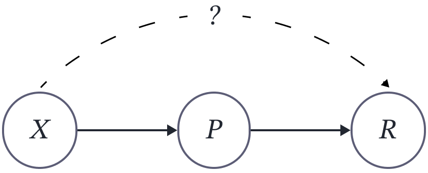
Figure 1. Standard stochastic $K$-armed bandit as a causal bandit.
Causal bandits extend the setting above by allowing the agent to receive additional information at the end of each round. This information comes in the form of samples from the Probabilistic Causal Model (PCM) to which the reward and action variables belong. More specifically, let $\mathcal{G}$ be a directed acyclic graph each node of which is associated with a random variable and let $\mathbb{P}$ be a distribution over the variables in the graph such that the following factorization holds:
\begin{align}
\mathbb{P}{\{\mathcal{V}}\}=\prod_{X\in\mathcal{V}}\mathbb{P}\{{X|\mathcal{P}(X)}\},
\end{align}
where $\mathcal{V}$ is the set of all the variables in the graph and $\mathcal{P}(X)$ is the set of parents of $X$. The pair $(\mathcal{G}\\,\mathbb{P})$ is the PCM and in this setting an agent interacts with it by performing interventions over sets of nodes $\mathbf{X}_t\subseteq\mathcal{V}$. An intervention cuts the incoming edges into the nodes in $\mathbf{X}_t$ and sets their values to the values $\mathbf{x}_t$ specified by the intervention. This results in a new probability distribution over the remaining nodes in the graph, denoted by ${\mathbb{P}\{\mathcal{V}\setminus\mathbf{X}_t\mid do (\mathbf{X}_t=\mathbf{x}_t)}\}$. As before, the goal of the agent is to maximize the expected total reward and the associated cumulative regret could be written as
\begin{align}
Reg_T(\mathcal{G},\mathcal{P})=\max_{\mathbf{X}\subseteq\mathcal{V’}}\max_{\mathbf{x}\in[K]^{\left| \mathbf{x} \right|}} \mu_{{\mathbf{X}}={\mathbf{x}}}-\sum_{t=1}^T\mathbb{E}[R_t],\tag{1}
\end{align}
where we denoted the set of parent nodes of the reward node by $\mathcal{P}$, assumed that each node in the graph takes on values from the set $[K]$, denoted with $\mathcal{V’}$ the set $\mathcal{V}\setminus{\{R}\}$, and introduced the notation $\mu_{\mathbf{X}=\mathbf{x}}$ for the expected value of the reward under the intervention $\ do (\mathbf{X}=\mathbf{x})$. In the regret definition we explicitly show the dependence on the graph and the sets of parents of the reward node. In general, the regret depends on the full definition of the PCM, including the probability distribution $\mathbb{P}$. This dependence is implicit in our notation. At the same time, the proposed algorithm will have dependence of the regret on the set of parent nodes which is why we include it in the notation here.

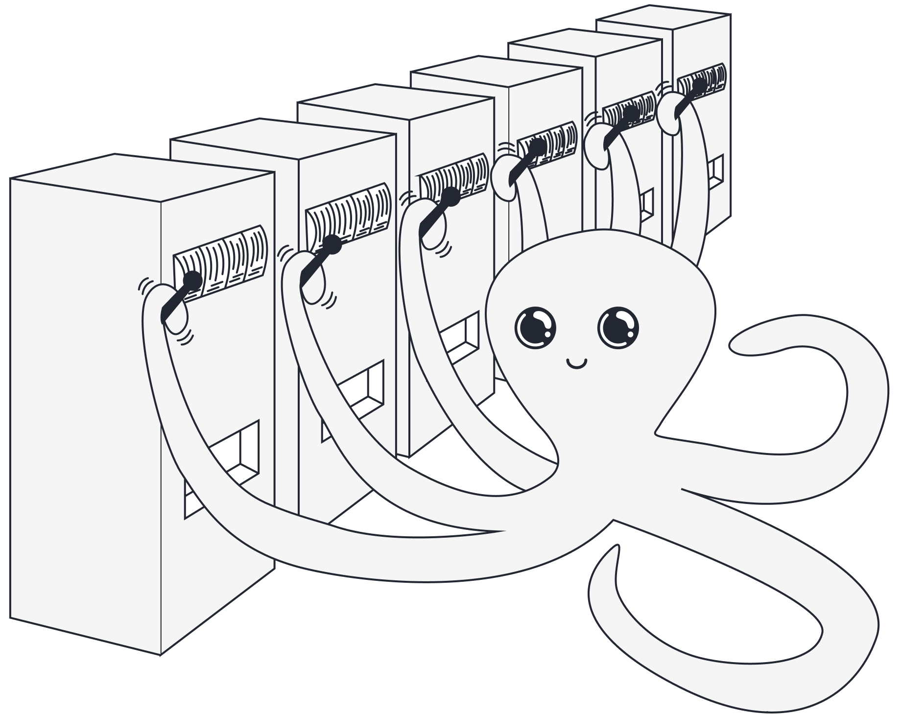
Octopus pulling leavers
Results from Bandit Literature
Standard stochastic $K$-armed bandit could be thought of as a causal bandit with the corresponding graph shown in Figure 1. At the same time, one could treat a causal bandit as a multi-armed bandit with $K^n$ arms. Define $\Delta_{\mathbf{X}=\mathbf{x}}$ as the reward gap of the action $\ do (\mathbf{X}=\mathbf{x})$ from the best action:
\begin{equation}
\Delta_{\mathbf{X}=\mathbf{x}} =\max_{\mathbf{Z}\subseteq\mathcal{V’}}\max_{\mathbf{z}\in[K]^{\left| \mathbf{Z} \right|}}\mu_{\mathbf{Z}=\mathbf{z}} -\mu_{\mathbf{X}=\mathbf{x}}.
\end{equation}
With this we can arrive at the following regret bound for causal bandits[1]:
\begin{align}
Reg_T(\mathcal{G},\mathcal{P})\preceq\sum_{\mathbf{X}\subseteq\mathcal{V’}}\sum_{\mathbf{x}\in[K]^{\left|{\mathbf{X}}\right|}} \Delta_{\mathbf{X}=\mathbf{x}}\left( {1+\frac{\log{T}}{\Delta_{\mathbf{X}=\mathbf{x}}^2}}\right).
\end{align}
Note however, that when $\Delta_{\mathbf{X}=\mathbf{x}}$ is small, the regret bound can become vacuous, since assuming that all the rewards are bounded, we get that the regret cannot grow faster than $\mathcal{O}(T)$. When $\Delta_{\mathbf{X}=\mathbf{x}}$ is small we can simply bound the regret by $\Delta_{\mathbf{X}=\mathbf{x}}T$ and using this [1] arrive at the following bound:
\begin{align}
Reg_T(\mathcal{G},\mathcal{P})\preceq\sum_{\textcolor{WildStrawberry}{\mathbf{X}\subseteq\mathcal{V’}}}\sum_{\textcolor{WildStrawberry}{\mathbf{x}\in[K]^{\left|{\mathbf{X}}\right|}}} \Delta_{\mathbf{X}=\mathbf{x}}+\sqrt{\textcolor{WildStrawberry}{K^n}T\log{T}}.
\end{align}
The dependence on $\textcolor{WildStrawberry}{K^n}$ is very bad and can itself lead to vacuous bound even for moderate values of $K$ and $n$. In our paper we aim to improve this dependence. In particular, [2] show that in the setting described in the previous section, the best intervention in the $PCM$ is over the set of the parent nodes of the reward node. Thus, we propose an algorithm that first discovers the set of parents of the reward node and then uses a standard multi armed bandit algorithm to discover the best interventions over the parents. When the number of parent nodes is smaller than the total number of nodes in the graph, this leads to an improvement.
Randomized Parent Search Algorithm
To find the parents of the reward node we first consider the case when there is at most one such parent. Consider the example in figure 2 that depicts a run of our algorithm on a graph with four nodes not including the reward node and a single parent of the reward node $P$. At each iteration the algorithm selects a node (shown in $\textcolor{gray}{gray}$) and intervenes on it to estimate the set of descendants of that node and whether the reward node is among these descendants. This is possible to do by comparing the observational distributions of all the nodes and mean reward value with the corresponding distributions and mean value under the intervention. If the current node is an ancestor of the reward node, the algorithm shall remove all the non-descendants of the current node from the consideration during the future iterations and otherwise it should focus only on the non descendants removing all the other nodes. In figure 2 $X_3$ is not an ancestor of $R$ and thus $X_3$ and its descendant $X_2$ should be removed from consideration. Subsequently, $X_1$ is an ancestor of $R$. It is possible that $X_1$ is a parent of $R$ and all its remaining descendants are not ancestors of $R$. Thus, the algorithm shall remember $X_1$ which is indicated by the question mark. At the next iteration there is only $P$ that is left and since it is an ancestor of $R$ that has no descendants, it should be returned as the estimated parent.

Figure 2. An example of a run of our algorithm to discover the parent node.
When there are multiple parents of the reward node our proposed algorithm discovers them one by one in a reverse topological order. Note that with the procedure described above, the algorithm shall discover a parent of the reward node that has no other parent of the reward node as its descendant. Thus, one could run a similar procedure to discover the next parent that may now have the first discovered parent as its descendant. There is a caveat, however, in that a node might be an ancestor of a previously discovered parent but not a parent of the reward node, see figure 3. In this case, intervening on this node will change the parent node, which in turn will change the reward node. To overcome this issue, our algorithm intervenes on all previously discovered parent nodes in addition to the node under consideration at each iteration. In the end, the procedure halts when there are no more parent nodes that could be discovered.

Figure 3. An example of a graph illustrating the need to intervene on previously discovered parents.
In practice, to determine the descendants of a node and whether the reward node is among them our algorithm requires to know the distribution and mean reward gaps which we will denote with $\epsilon$ and $\Delta$. These are the smallest absolute values of the difference between the distribution (mean) for intervention when discovering a new parent from the distribution (mean) when discovering the previous parent or observational distribution during the time when trying to discover the first parent. We refer the reader to the paper for the full formal definition. The algorithm compares the empirical values of the gaps with their true values and determines that a node is a descendant of the current node under consideration when the empirical gap is at most $\epsilon/2$. Similarly, it determines that the reward node is a descendant of the current node, when the empirical mean threshold is below $\Delta/2$.
The full algorithm is presented in algorithm 1 and maintains
- the set of previously discovered parents $\mathcal{\hat{P}}$,
- the last discovered ancestor of $R$ denoted by $\hat{P}$ (corresponds to the question mark in figure 2),
- the
candidate setof nodes $\mathcal{C}$, and the descendants of $\hat{P}$ denoted $\mathcal{D’}$ (corresponds to the set of not crossed out nodes in figure 2), and - a set of nodes $\mathcal{S}$ that should be excluded from consideration when trying to find the next parent.
After intervening on the current node and all the nodes in the set of parents found up until the current iteration of the while loop on lines 6-9, the algorithm estimates the descendants of the selected node $X$ on line 10. The test on line 11 determines whether the current node is an ancestor of $R$ and after that the sets $\mathcal{S},\mathcal{C},\mathcal{D’}$ and the value of $\hat{P}$ are updated accordingly. After that if there are no nodes in the candidate set $\mathcal{C}$ then $\hat{P}$ must denote the new parent. If all parents have already been discovered then $\hat{P}$ will take on the $\texttt{null}$ value denoted by $\varnothing$.
Regret Bound of our Approach
Denote with $\textcolor{MidnightBlue}{\mathbb{E}[N(\mathcal{G},\mathcal{P})]}$ the expected number of distinct node interventions required to discover the parent nodes with our algorithm and $E$ be the event that the set of discovered parent nodes is equal to the true set of parent nodes. We provide a high probability guarantee for the event $E$ to hold and as a result a high probability conditional regret bound of our approach where the expected total reward is conditioned on $E$.
Algorithm 1 Full version of $RAPS$ for unknown number of parents
Require: Set of nodes $\mathcal{V}$ of $\mathcal{G}$, $\epsilon,\Delta$, probability of incorrect parent set estimate $\delta$
Output: Estimated set of parent nodes $\mathcal{\hat{P}}$
1: $\mathcal{\hat{P}} \gets\emptyset$, $\mathcal{S} \gets\emptyset$, $\hat{P}\gets\varnothing$, $\mathcal{C} \gets\mathcal{C}$, $\mathcal{D’} \gets\emptyset$
# $\mathcal{D’}$ is the set of descendants of last ancestor of $R$
2: $B\gets\max\left\{ {\frac{32}{\Delta^2}\log\left( {\frac{8nK(K+1)^n}{\delta}} \right),
\frac8{\epsilon^2}\log\left( {\frac{8n^2K^2(K+1)^n}{\delta}} \right)} \right\}$
3: Observe $B$ samples from $PCM$ and compute $\bar{R}$ and $\hat{P}(X)$ for all $X\in\mathcal{V}$
4: while $\mathcal{C}\neq\emptyset$ do
5: $\qquad X\sim Unif(\mathcal{C})$
6: $\qquad$ for $x\in[K]$ and $\mathbb{z}\in[K]^{\left| {\mathcal{\hat{P}}} \right|}$ do
7: $\qquad\qquad$ Perform $B$ interventions $do (X=x,\mathcal{\hat{P}}=\mathbf{z})$
8: $\qquad\qquad$ Compute $\bar{R}^{do (X=x,\mathcal{\hat{P}}=\mathbf{z})}$, $\hat{P}(Y| do (X=x,\mathcal{\hat{P}}=\mathbf{z}))$ for all $Y\in\mathcal{V}$
9: $\qquad$ end for
10: $\qquad$Estimate descendants of $X$:
\begin{align*}
\mathcal{D}\gets\biggl\{Y\in\mathcal{V} &\mid \exists x\in[K],\mathbf{z}\in[K]^{\left| {\mathcal{\hat{P}}} \right|}, \\ &\text{ such that }\left| {\hat{P}(Y|do(\mathcal{\hat{P}}=\mathbf{z})) -\hat{P}(Y|do(X=x,\mathcal{\hat{P}}=\mathbf{z}))} \right|>\epsilon/2\biggr\}
\end{align*}
11: $\qquad$ if $\exists x\in[K],\mathbf{z}\in[K]^{\left| {\mathcal{\hat{P}}} \right|}$ such that $\left| {\bar{R}^{do(\mathcal{\hat{P}}=\mathbf{z})}-\bar{R}^{do(X=x,\mathcal{\hat{P}}=\mathbf{z})}} \right| > \Delta/2$ then
12: $\qquad\qquad \mathcal{C}\gets\mathcal{D}\setminus\left\{ {X} \right\}$
13: $\qquad\qquad \mathcal{\hat{P}}\gets X, \mathcal{D’}\gets\mathcal{D}$
14: $\qquad$ else
15: $\qquad\qquad \mathcal{C}\gets\mathcal{C}\setminus \mathcal{D}$
16: $\qquad\qquad \mathcal{S}\gets\mathcal{S}\cup\mathcal{D}$
17: $\qquad$ end if
18: $\qquad$ if $\mathcal{C}=\emptyset$ and $\mathcal{\hat{P}}\neq\varnothing$ then
19: $\qquad\qquad \mathcal{\hat{P}}\gets\mathcal{\hat{P}}\cup\left\{ {\hat{P}} \right\}$
20: $\qquad\qquad \mathcal{S}\gets\mathcal{S}\cup\mathcal{D’}$
21: $\qquad\qquad \mathcal{C}\gets\mathcal{V}\setminus\mathcal{S}$
22: $\qquad\qquad \mathcal{\hat{P}}\gets\varnothing$
23: $\qquad$ end if
24: end while
25: return $\mathcal{\hat{P}}$
Theorem 1. For the learner that uses algorithm 1 and then runs $UCB$ the following bound for the conditional regret holds with probability at least $1-\delta$:
\begin{equation}
Reg_T(\mathcal{G},\mathcal{P}\mid E)\preceq \max\left\{ {\textcolor{Orange}{ \frac1{\Delta^2},\frac1{\epsilon^2}}} \right\} \textcolor{WildStrawberry}{ K^{\left| \mathcal{P} \right|+1}}\textcolor{MidnightBlue}{\mathbb{E}[N(\mathcal{G},\mathcal{P})]}\log \left( { \frac{\textcolor{WildStrawberry}{nK^n}}{\delta}} \right) +\sum_{\textcolor{WildStrawberry}{\mathbf{x}\in[K]^{\left| {\mathcal{P}} \right|}}} \Delta_{\mathcal{P}=\mathbf{x}} \left( {1+\frac{\log{T}}{\Delta_{\mathcal{P}=\mathbf{x}}^2} }\right).
\end{equation}
In the bound above we see improved dependence from $K^n$ to $K^{\left|{\mathcal{P}}\right|+1}$ which leads to improved performance of our algorithm when the number of parents is small. We hypothesize that $\max{\{\textcolor{Orange}{1/\Delta^2}, \textcolor{Orange}{1/\epsilon^2}}\}$ dependence is suboptimal and could be improved. For the expected number of distinct node interventions we prove the following result.
Theorem 2. Let $\mathcal{P}=\left\{ P \right\}$, then the number of distinct node interventions for
any graph $\mathcal{G}$ is equal to:
\begin{equation}
\textcolor{MidnightBlue}{\mathbb{E}[N(\mathcal{G},P)]}
=\sum_{X\in\mathcal{V’}}\frac1{\left| \mathcal{A}(X)\triangle\mathcal{A}(P)\cup\left\{ {X} \right\} \right|},
\end{equation}
where $\mathcal{A}(X)$ is the set of ancestors of $X$ in the graph induced over the nodes in $\mathcal{V’}$ and $A\triangle B$ stands for the symmetric difference of sets $A$ and $B$, i.e. $A\triangle B=(A\cup B)\setminus(A\cap B)$.

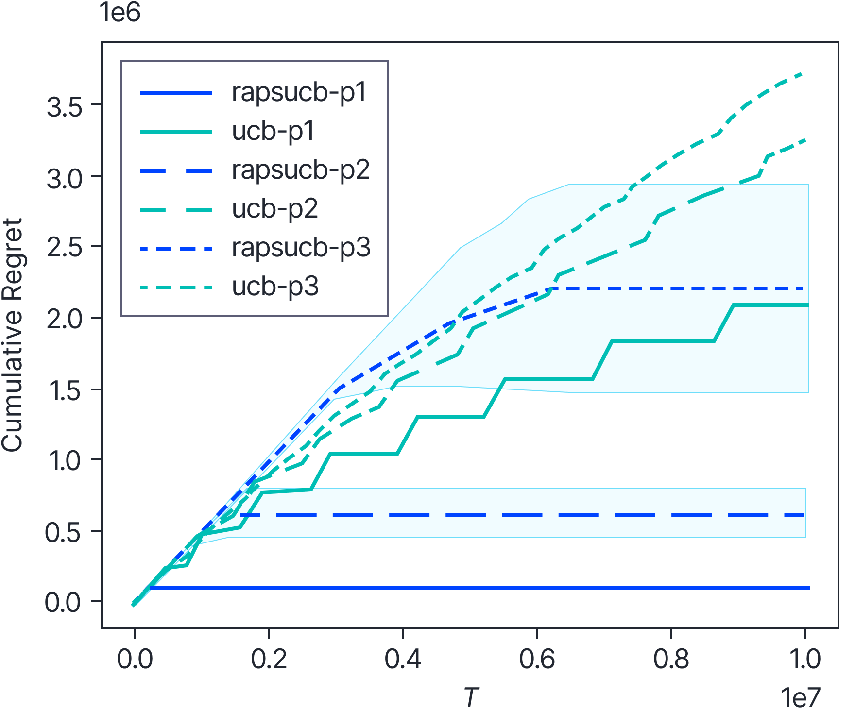
Figure 4. Regret of $RAPS$+$UCB$ vs $UCB$ on a tree graphover $\mathcal{V’}$ with the number of parents ranging from 1 to 3 indicated by the last character in the label.
In the paper we provide conditions under which the expected number of distinct node interventions to discover the parent node is sublinear and also extend these conditions to the case when the reward node has multiple parents.
Experimental Verification
In figure 4 we empirically verify that our approach achieves an improvement. For this figure we let the graph have a binary tree structure for which our theory predicts $\Theta\left({\frac{n}{\log_2{n}}}\right)$ number of distinct node interventions. While this graph structure does not lead to the best number of distinct node interventions, we still expect to see an improvement since discovering the set of parent nodes drastically reduces the set of arms that $UCB$ has to explore.
Conclusion
In this blog post we introduced a causal bandit problem and proposed an algorithm that combines randomized parent search and standard $UCB$ algorithm to achieve improved regret. Check out the full paper for mode details. We would also like to note that possible directions for future work included improving the dependence on $\epsilon$ and $\Delta$, lifting the assumption of no unobserved confounders and proving lower bounds for causal bandits with unknown graph structure.
References
[1] Tor Lattimore and Csaba Szepesv ́ari. Bandit algorithms. Cambridge University Press, 2020.
[2] Sanghack Lee and Elias Bareinboim. Structural causal bandits: where to intervene? Advances in Neural Information Processing Systems, 31, 2018.