Adversarial contrastive estimation: harder, better, faster, stronger

Summary: Many machine learning models train by the process of trying to separate positive examples (i.e., something true and physically observed) found in real data from “fictitious” negative examples (i.e., any other configuration that’s not actually observed in the data). To train, you need both positive and negative examples, and while positive examples are easily accessible because they’re already from your dataset, it becomes necessary to construct the negative examples by design. However, the construction of negative examples has historically suffered from subpar quality because their design choice was often motivated by computational reasons. 

One of the ways of constructing these “easy” negative examples is through Noise Contrastive Estimation (NCE), a method that randomly samples configurations for negative examples. But by only sampling easy negative examples, the model fails to learn discriminating features and consequently leads to a poor final performance. In this work, we show the need for hard negative examples and provide a method to generate them. We propose to augment the negative sampler in NCE with an adversarially learned adaptive sampler that finds harder negative examples. Our method, dubbed Adversarial Contrastive Estimation (ACE), leads to improvements over a wide array of embedding models that validate the generality of the approach. 

Background on Contrastive Learning

Contrastive Learning operates by contrasting losses on positive and negative examples. By seeing both these types of data, the model can try to distinguish between the two. A few popular approaches include the aforementioned Noise Contrastive Estimation (NCE) to train a skip-gram model for word embeddings, and triplet loss for deep metric learning. Again, positive examples are taken from the real data distribution i.e., training set, while negative examples are any configurations of data that are not directly observed in real data. In their most general form, contrasting learning problems can be framed as follows:

\begin{equation}
\label{general_loss}
L(\omega) = E_{p(x^+,y^+,y^-)} l_{\omega}(x^+,y^+,y^-)
\end{equation}

Here l_ω(x⁺,y⁺,y⁻) captures both the model with parameters ω and the loss that scores a positive tuple (x⁺,y⁺) against a negative one (x⁺,y⁻). E_{p (x⁺,y⁺,y⁻)}(.) denotes expectation with respect to some joint distribution over positive and negative samples. With a bit of algebra and the fact that given x⁺, the negative sampling is not dependent on the positive label, we can simplify the expression to E_p(x⁺)[E_{p(y⁺|x⁺)p(y⁻|x⁺)}l_ω(x⁺,y⁺,y^–)]. In some cases, the loss can be written as a sum of scores on positive and negative tuples. This is the case with NCE in word embeddings when using cosine similarity as the scoring function. In other cases, the loss is not decomposable as with a max margin objective, but that won’t deter our treatment. 

Noise Contrastive Estimation

NCE can be viewed as a special case of our factorized general loss where p(y⁻|x⁺) is taken from a predefined noise distribution. For example, in the case of word embeddings, this could mean picking a centre word as x⁺ and then randomly sampling a word from the entire vocabulary set y^– rather than using the context word, which in our notation would be y⁺. The idea is that the negative sampled word is unlikely to form a word-context pair that would actually be observed in the real data distribution. 

What’s wrong with this approach?

The negatives produced from a fixed distribution are not tailored towards x⁺ so they’re likely to be too easy. The problem with this approach is that the model fails to continuously improve throughout the entirety of training due to the absence of hard negative examples. As training progresses, and more and more negative examples are correctly learned, the probability of drawing a hard negative example (see definition below) further diminishes, thus causing slow convergence.

Adversarial Contrastive Estimation

Before we talk about ACE and its benefits, we need to first clarify what we mean by hard negative examples. For us, hard negative examples are datapoints that are extremely difficult for the training model to distinguish from positive examples. Hard negative examples necessarily result in higher losses during training, which is useful because when you have higher losses, you get more informative gradients that aid in training. We can take inspiration from conditional generative adversarial networks (CGAN), as we intuitively want to sample negative configurations that can “fool” the model into thinking they were sampled from the real data distribution. However, it is important to note that at the beginning of training, the model needs a few easy examples to get off the ground. Thus, we can augment NCE with an adversarial sampler of the following form: λp_nce(y⁻) + (1−λ)g_θ(y⁻|x⁺), where g_θ is a conditional distribution with a learnable parameter θ and λ is a hyperparameter. The overall objective function can then be stated as:

\begin{align}
\label{ace_value_general}
L(\omega, \theta; x) = \lambda E_{p(y^+|x)p_{nce}(y^-)} l_{\omega}(x,y^+,y^-) \nonumber +(1-\lambda) E_{p(y^+|x)g_\theta(y^-|x)}l_{\omega}(x,y^+,y^-)
\end{align}

Learning can then proceed if we recognize the main model as the discriminator and the adversarial negative sampler as the generator in a GAN-like setup. However, one slight distinction from a regular GAN is that the generator g_θ(y^–|x⁺) defines a categorical distribution over possible y⁻ values, and samples are drawn accordingly. As a result, the generator picks an action that is a discrete choice, which prevents gradients from flowing back. The generator’s reward is based on its ability to fool the discriminator into thinking the negative samples produced are positive ones. We appeal to the policy gradient literature to train our generator. Specifically, we used the REINFORCE gradient estimator, which is perhaps the simplest one. Another difference is that in cGAN, we would like to find an equilibrium where the generator wins, whereas here, we want the discriminator to win. To ensure that the min-max optimization leads to a saddle point where the discriminator learns good representation of data, we introduce a number of training techniques.

Training Tricks

GAN training is notorious for being unstable and when paired with reinforcement learning methods, this phenomenon gets exacerbated. Here are few tricks we used that helped to effectively train with ACE:

• Entropy Regularizer: We found that the generator often collapsed to its favourite set of negative examples, which prevented the model from improving further. To fix this problem, we added a small term to the generator’s loss to ensure it maintained high entropy. The term: R_ent(x)=max(0,c−H(g_θ(y|x))) contains H which is the entropy of the categorical distribution and c=log(k) is the entropy of a uniform distribution over k choices, while k is a hyperparameter.

Observation: This worked most of the time and never hurt the overall performance.

• Handling False Negatives: When the action space is small, the generator can occasionally sample negatives which leads to a positive example and therefore a false negative result. In NCE, this tends to occur but is not a severe problem as the sampling is random. In ACE, this could be a serious problem as the generator could collapse to these false negatives. Whenever computationally feasible, we apply an additional two-step technique. First, we maintain a hash map of the training data in memory, and use it to efficiently detect if a negative sample (x⁺,y⁺) is an actual observation then filter it out. 

Observation: This is helpful for tasks such knowledge graphs and order embeddings, but not feasible for word embeddings where the vocabulary size is large.

• Variance Reduction: REINFORCE is known to have extremely high variance. To fix this problem we used the self-critical baseline. 

Observation: This only seemed to help with the word embedding task.

• Importance Sampling using NCE: The generator can leverage NCE samples for exploration in an off-policy scheme. One way to do this is to use importance re-weighting to take advantage of the NCE samples that weren’t chosen by the generator. This results in a modified reward of g_θ(y⁻|x)/p_nce(y⁻).

Observation: Surprisingly, this technique rarely worked well and we’re not quite sure why, since theoretically it is supposed to work. 

Experimental Results

We tested ACE on 3 different embedding tasks: Word Embeddings, Order Embeddings, and Knowledge Graph Embeddings. You can check out our paper for a more detailed analysis, but the moral of the story is that whenever learning required a contrastive objective, ACE worked better than NCE, in fact, it usually lifts simple baseline models to be competitive with or superior to SOTA.

Word Embeddings on Wikipedia

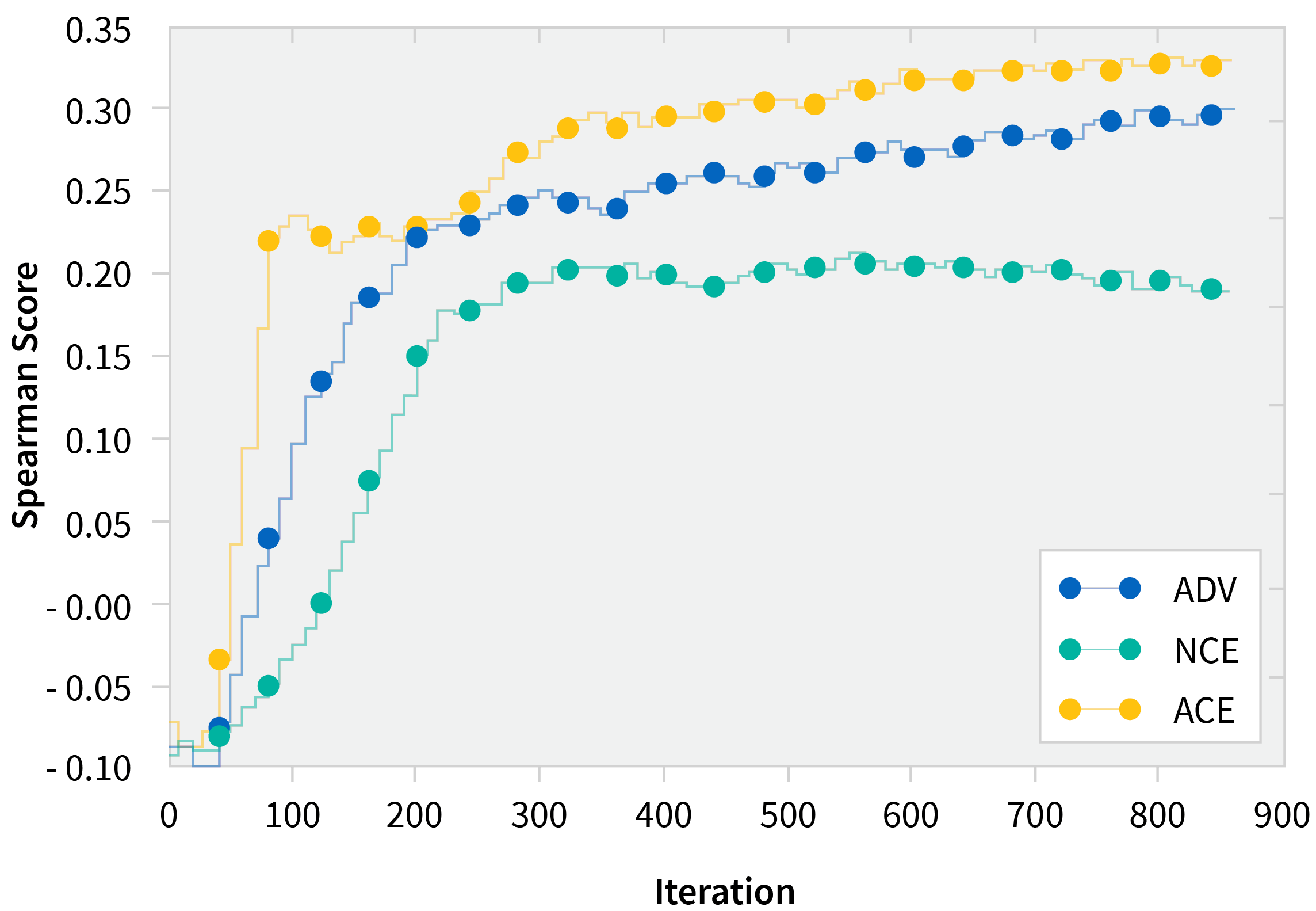
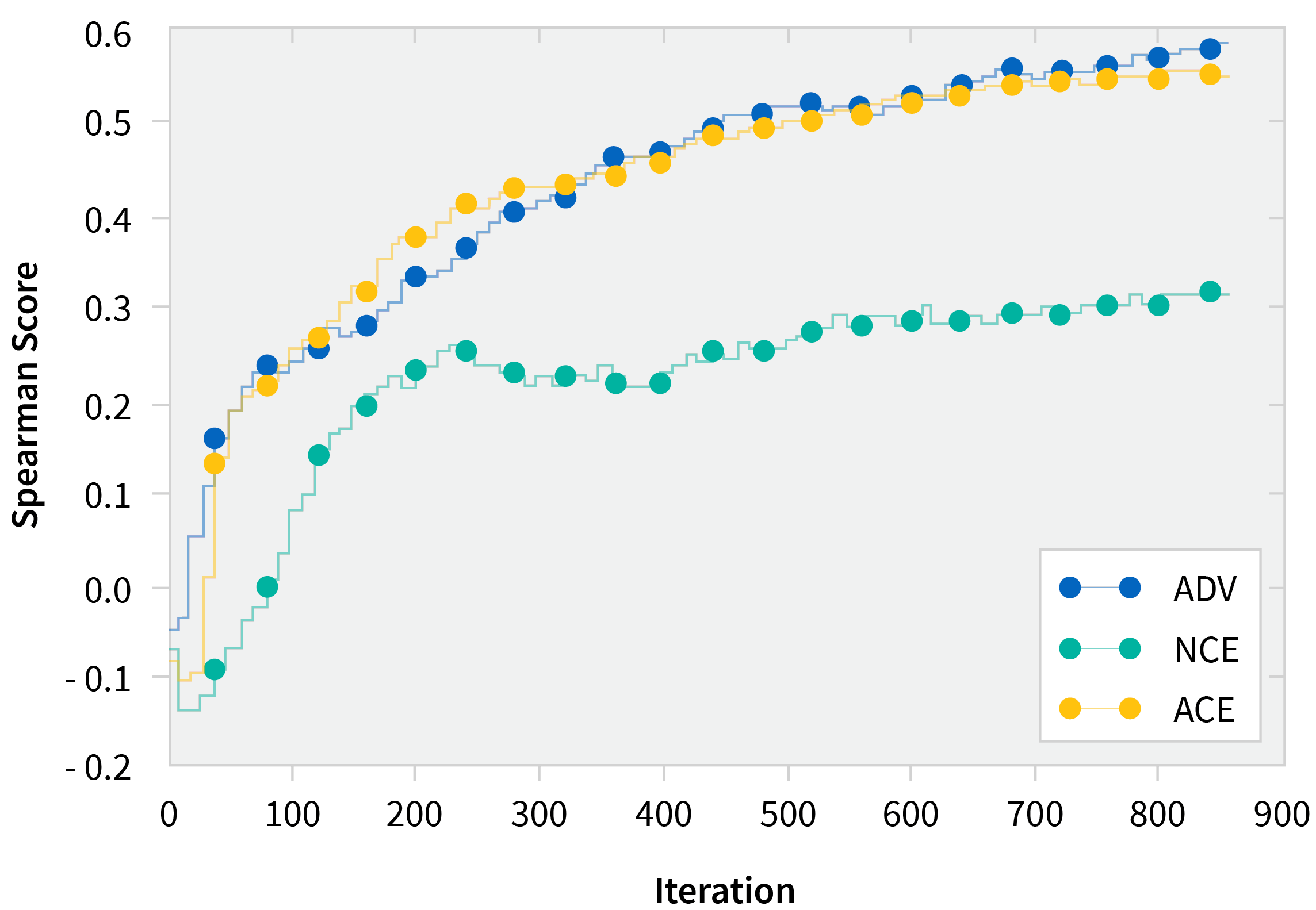
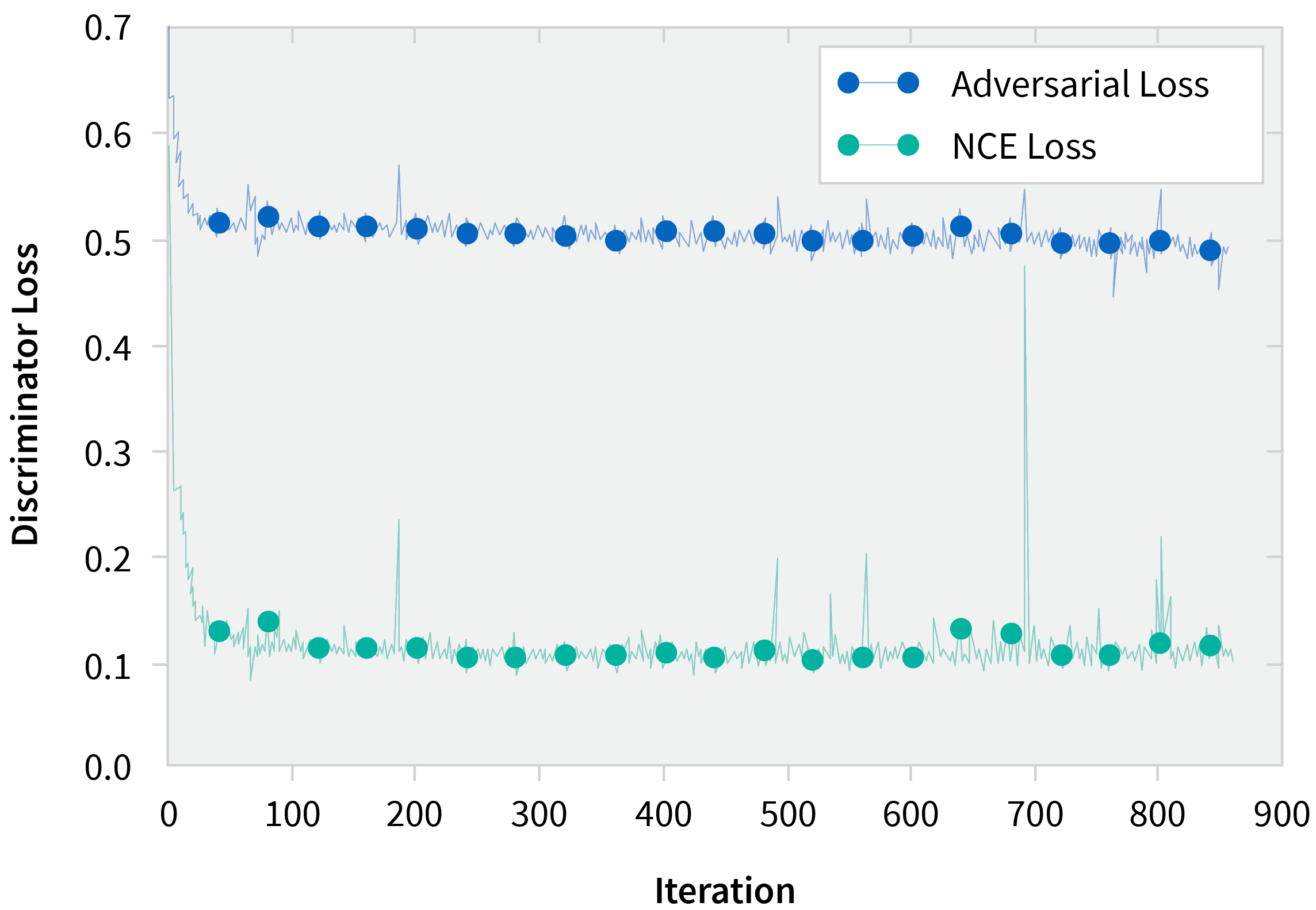
As expected when using ACE, we saw that learning was more sample efficient and often converged to higher values than just vanilla NCE. We also validated the hypothesis that ACE samples were harder based on the third plot (see graph below), which shows a higher loss incurred by ACE samples than their NCE counterparts.

Spearman Score on Stanford Rareword Dataset

Spearman Score on WordSim-353 Dataset

Discriminator Loss on Adversarial and NCE Samples 

Ablation Study with Knowledge Graph Embeddings

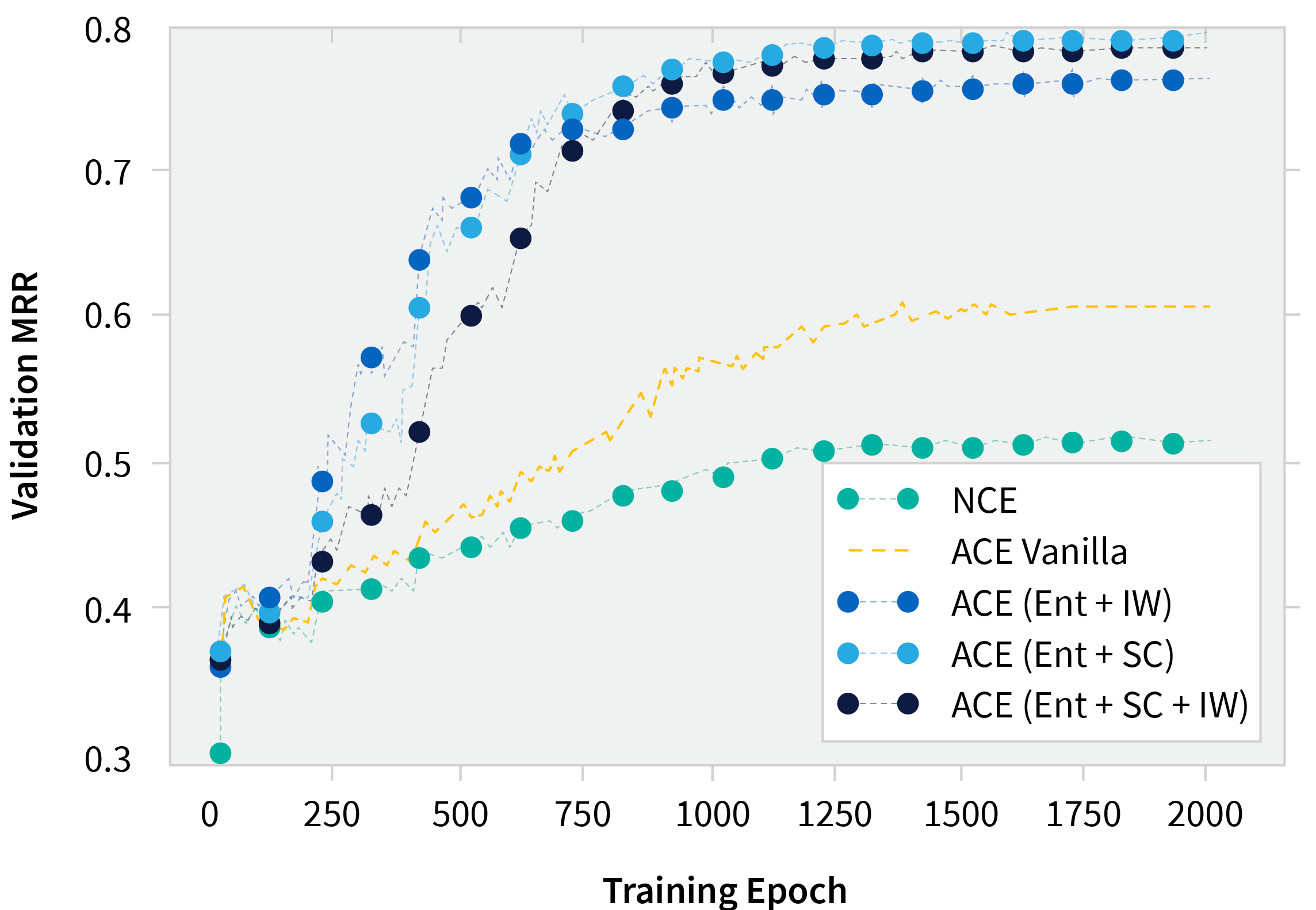
We also did an ablation study using the various training tricks listed above on learning knowledge graph embeddings. The punchline is this: ACE always worked better than NCE and entropy regularization was critical for this task.

Limitations and Discussion

The generator needed to construct a categorical distribution over all possible actions in order to sample, but this can be very expensive if the action space is very large. While ACE ended up being more sample efficient, it may not be faster in terms of wall-clock time. However, most embedding models are usually geared toward some downstream task [i.e., word embeddings] in language models, so we argue that spending more time on a better embedding model via ACE is worth the effort. Another limitation that results from using ACE is that with the adversarial generator, we lost the guarantee of Maximum Likelihood Estimation (MLE). MLE is provided by NCE as an asymptotic limit, but this is true for any GAN-based method and currently, to the best of our knowledge, there aren’t sufficient tools for analyzing the equilibrium of a min-max game where players are parametrized by deep neural nets. 

TL;DR

Regardless of the problem or dataset, if learning resembles a contrastive objective, ACE works by sampling Harder negatives which leads to Better convergence while being Faster in the number of samples seen and results in an overall Stronger model. 

Acknowledgments

The authors would like to thank Prof. Matt Taylor and Prof. Jackie Cheung for helpful feedback. Jordana Feldman for help with writing. Also, an immense thank you to April Cooper for the gorgeous visuals. Finally, countless others for the espresso talks, you know who you are.