
Introduction
Discrimination is the unequal treatment of individuals of certain groups, resulting in members of one group being deprived of benefits or opportunities. Common groups that suffer discrimination include those based on age, gender, skin colour, religion, race, language, culture, marital status, or economic condition.
The unintentional unfairness that occurs when a decision has widely different outcomes for different groups is known as disparate impact. As machine learning algorithms are increasingly used to determine important real-world outcomes such as loan approval, pay rates, and parole decisions, it is incumbent on the AI community to minimize unintentional discrimination.
This tutorial discusses how bias can be introduced into the machine learning pipeline, what it means for a decision to be fair, and methods to remove bias and ensure fairness.
Where does bias come from?
There are many possible causes of bias in machine learning predictions. Here we briefly discuss three: (i) the adequacy of the data to represent different groups, (ii) bias inherent in the data, and (iii) the adequacy of the model to describe each group.
Data adequacy. Infrequent and specific patterns may be down-weighted by the model in the name of generalization and so minority records can be unfairly neglected. This lack of data may not just be because group membership is small; data collection methodology can exclude or disadvantage certain groups (e.g., if the data collection process is only in one language). Sometimes records are removed if they contain missing values and these may be more prevalent in some groups than others.
Data bias. Even if the amount of data is sufficient to represent each group, training data may reflect existing prejudices (e.g., that female workers are paid less), and this is hard to remove. Such historical unfairness in data is known as negative legacy. Bias may also be introduced by more subtle means. For example, data from two locations may be collected slightly differently. If group membership varies with location this can induce biases. Finally, the choice of attributes to input into the model may induce prejudice.
Model adequacy. The model architecture may describe some groups better than others. For example, a linear model may be suitable for one group but not for another.
Definitions of fairness
A model is considered fair if errors are distributed similarly across protected groups, although there are many ways to define this. Consider taking data $\mathbf{x}$ and using a machine learning model to compute a score $\mbox{f}[\mathbf{x}$$]$ that will be used to predict a binary outcome $\hat{y}\in\{0,1\}$. Each data example $\mathbf{x}$ is associated with a protected attribute $p$. In this tutorial, we consider it to be binary $p\in\{0,1\}$. For example, it might encode sub-populations according to gender or ethnicity.
We will refer to $p=0$ as the deprived population and $p=1$ as the favored population. Similarly we will refer to $\hat{y}=1$ as the favored outcome, assuming it represents the more desirable of the two possible results.
Assume that for some dataset, we know the ground truth outcomes $y\in\{{0,1}\}$. Note that these outcomes may differ statistically between different populations, either because there are genuine differences between the groups or because the model is somehow biased. According to the situation, we may want our estimate $\hat{y}$ to take account of these differences or to compensate for them.
Most definitions of fairness are based on group fairness, which deals with statistical fairness across the whole population. Complementary to this is individual fairness which mandates that similar individuals should be treated similarly regardless of group membership. In this blog, we’ll mainly focus on group fairness, three definitions of which include: (i) demographic parity, (ii) equality of odds, and (iii) equality of opportunity. We now discuss each in turn.
Demographic Parity
Demographic parity or statistical parity suggests that a predictor is unbiased if the prediction $\hat{y}$ is independent of the protected attribute $p$ so that
\begin{equation}
Pr(\hat{y}|p) = Pr(\hat{y}). \tag{2.1}
\end{equation}
Here, the same proportion of each population are classified as positive. However, this may result in different false positive and true positive rates if the true outcome $y$ does actually vary with the protected attribute $p$.
Deviations from statistical parity are sometimes measured by the statistical parity difference
\begin{equation}
\mbox{SPD} = Pr(\hat{y}=1 | p=1) – Pr(\hat{y}=1 | p=0), \tag{2.2}
\end{equation}
or the disparate impact which replaces the difference in this equation with a ratio. Both of these are measures of discrimination (i.e. deviation from fairness).
Equality of odds
Equality of odds is satisfied if the prediction $\hat{y}$ is conditionally independent to the protected attribute $p$, given the true value $y$:
\begin{equation}
Pr(\hat{y}|y,p) = Pr(\hat{y}| y). \tag{2.3}
\end{equation}
This means that the true positive rate and false positive rate will be the same for each population; each error type is matched between each group.
Equality of opportunity
Equality of opportunity has the same mathematical formulation as equality of odds, but is focused on one particular label $y=1$ of the true value so that:
\begin{equation}
Pr(\hat{y}|y=1,p) = Pr(\hat{y}| y=1). \tag{2.4}
\end{equation}
In this case, we want the true positive rate $Pr(\hat{y}=1|y=1)$ to be the same for each population with no regard for the errors when $y=0$. In effect it means that the same proportion of each population receive the “good” outcome $y=1$.
Deviation from equality of opportunity is measured by the equal opportunity difference:
\begin{equation}
\mbox{EOD} = Pr(\hat{y}=1 | y=1, p=1) – Pr(\hat{y}=1 | y=1, p=0). \tag{2.5}
\end{equation}
Worked example: loans
To make these ideas concrete, we consider the example of an algorithm that predicts credit rating scores for loan decisions. This scenario follows from the work of Hardt et al. (2016) and the associated blog.
There are two pools of loan applicants $p\in\{{0,1}\}$ that we’ll describe as the blue and yellow populations. We assume that we are given historical data, so we know both the credit rating and whether the applicant actually defaulted on the loan ($y=0$) or repaid it ($y=1$).
We can now think of four groups of data corresponding to (i) the blue and yellow populations and (ii) whether they did or did not repay the loan. For each of these four groups we have a distribution of credit ratings (figure 1). In an ideal world, the two distributions for the yellow population would be exactly the same as those for the blue population. However, as figure 1 shows, this is clearly not the case here.

Figure 1. Loan example setup. We consider two populations: blue (protected attribute $p=0$) and yellow (protected attribute $p=1$) a) Empirically observed distributions of credit rating scores produced by a machine learning algorithm for the blue population for the cases where they either defaulted on the loan (dashed line) or paid it back (solid line). b) Empirically observed distributions for the yellow population. Note that the distributions differ in weighting, mean position and overlap for the blue and yellow groups.
Why might the distributions for blue and yellow populations be different? It could be that the behaviour of the populations is identical, but the credit rating algorithm is biased; it may favor one population over another or simply be more noisy for one group. Alternatively, it could be that that the populations genuinely behave differently. In practice, the differences in blue and yellow distributions are probably attributable to a combination of these factors.
Let’s assume that we can’t retrain the credit score prediction algorithm; our job is to adjudicate whether each individual is refused the loan ($\hat{y}=0)$ or granted it ($\hat{y}=1$). Since we only have the credit score $\mbox{f}[\mathbf{x}$$]$ to go on, the best we can do is to assign different thresholds $\tau_{0}$ and $\tau_{1}$ for the blue and yellow populations so that the loan is granted if $f[\mathbf{x}$$]$ $>\tau_{0}$ for the blue population and $f[\mathbf{x}$$]$ $>\tau_{1}$ for the yellow population.
Comparison of fairness criteria
We’ll now consider different possible ways to set these thresholds that result in different senses of fairness. We emphasize that we are not advocating any particular criterion, but merely exploring the ramifications of different choices.
Blindness to protected attribute: We choose the same threshold for blue and yellow populations. This sounds sensible, but it neither guarantees that the overall frequency of loans, nor the frequency of successful loans will be the same for the two groups. For the thresholds chosen in figure 2a, many more loans are made to the yellow population than the blue population (figure 2b). Moreover, examination of the receiver operating characteristic (ROC) curve shows that both the rate of true positives $Pr(\hat{y}=1|y=1)$ and false alarms $Pr(\hat{y}=1|y=0)$ differ for the two groups (figure 2c).
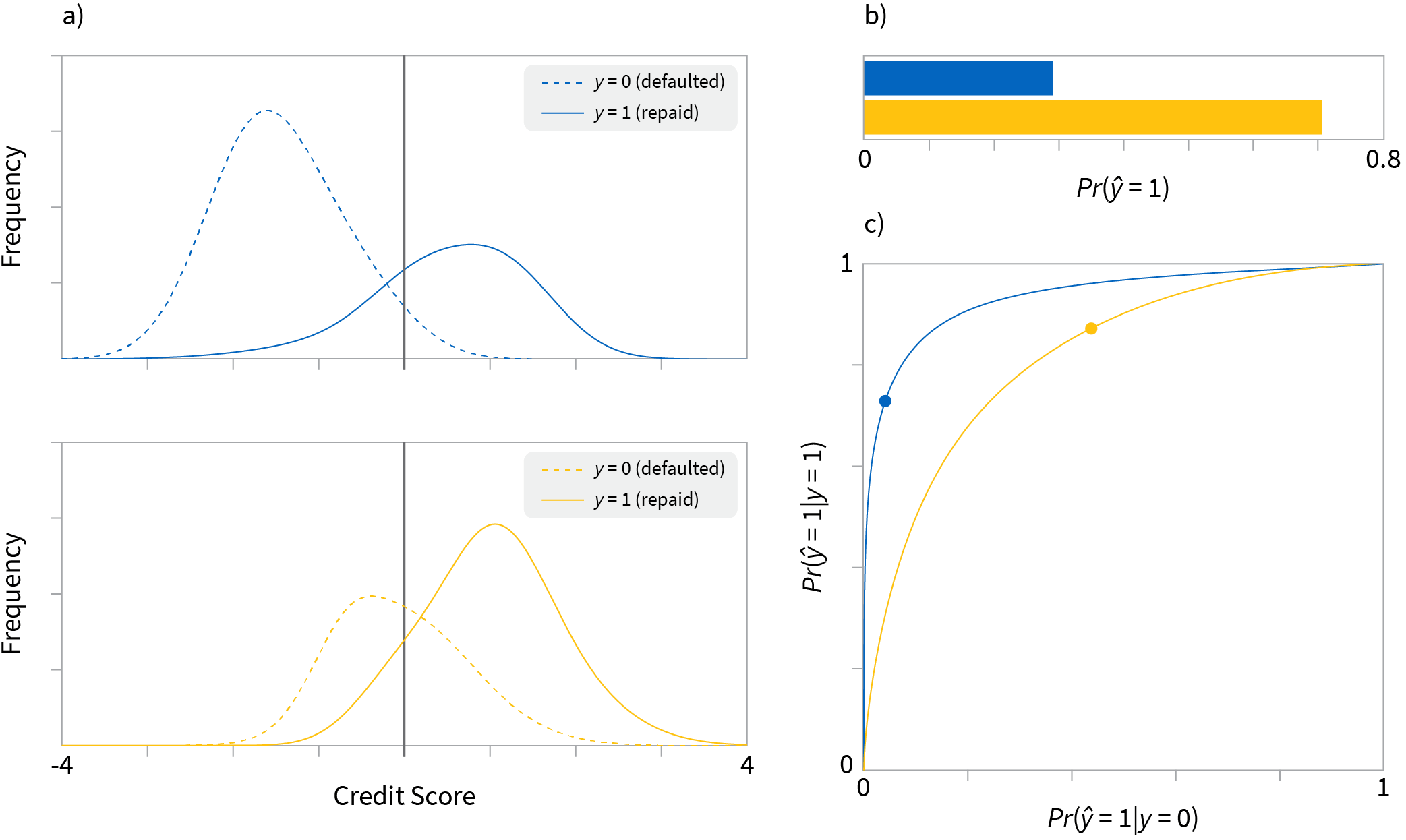
Figure 2. Blindness to protected attribute. a) If we ignore the protected attribute and set the thresholds (black solid lines) to be the same for both blue and yellow populations, then fairness is not achieved. b) The overall positive rate $Pr(\hat{y})$ (proportion of people given loans regardless of outcome) is not the same in each population. c) ROC curves for the curves (points represent chosen thresholds). The true positive rate $Pr(\hat{y}=1|y=1)$ (proportion of people who were offered loan and paid it back successfully) is not the same for each population either as shown by the different vertical positions of the points on the ROC curves.
Equality of odds: This definition of fairness proposes that the false positive and true positive rates should be the same for both populations. This also sounds reasonable, but figure 2c shows that it is not possible for this example. There is no combination of thresholds that can achieve this because the ROC curves do not intersect. Even if they did, we would be stuck giving loans based on the particular false positive and true positive rates at the intersection which might not be desirable.
Demographic parity: The threshold could be chosen so that the same proportion of each group are classified as $\hat{y} =1$ and given loans (figure 3). We make an equal number of loans to each group despite the different tendencies of each to repay (figure 3b). This has the disadvantage that the true positive and false positive rates might be completely different in different populations (figure 3c). From the perspective of the lender, it is desirable to give loans in proportion to people’s ability to pay them back. From the perspective of an individual in a more reliable group, it may seem unfair that the other group gets offered the same number of loans despite the fact they are less reliable.
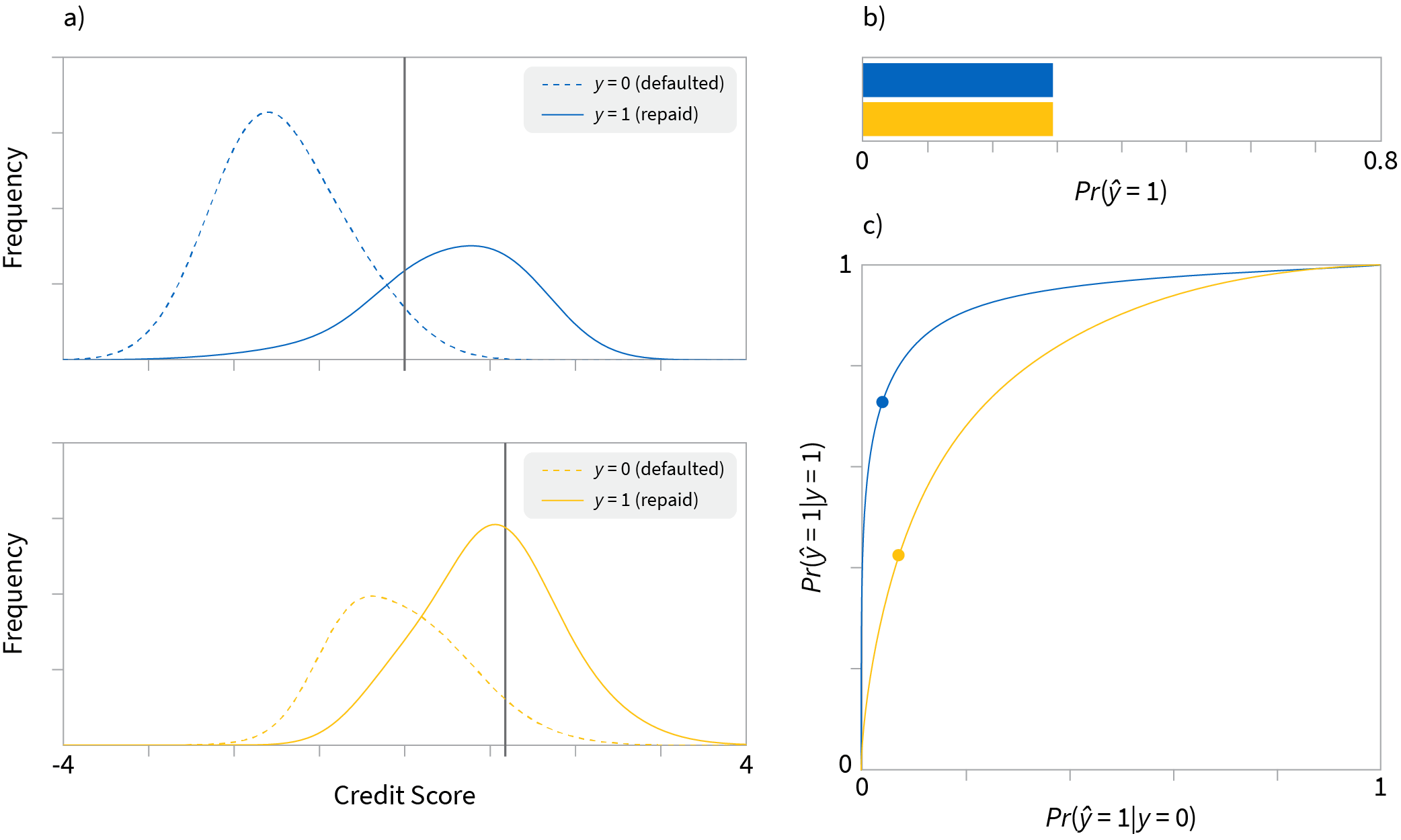
Figure 3. Demographic parity. a) We carefully choose different thresholds for each population so that b) the same proportion of the each group are given loans. This has the disadvantage that the true positive rate $Pr(\hat{y}=1|y=1)$ proportion of people who are given loans and did pay them back are different between each group (points on ROC curve are at different heights).
Equal opportunity: The thresholds are chosen so that so that the true positive rate is is the same for both population (figure 4). Of the people who pay back the loan, the same proportion are offered credit in each group. In terms of the two ROC curves, it means choosing thresholds so that the vertical position on each curve is the same without regard for the horizontal position (figure 2c). However, it means that different proportions of the blue and yellow groups are given loans (figure 4b).
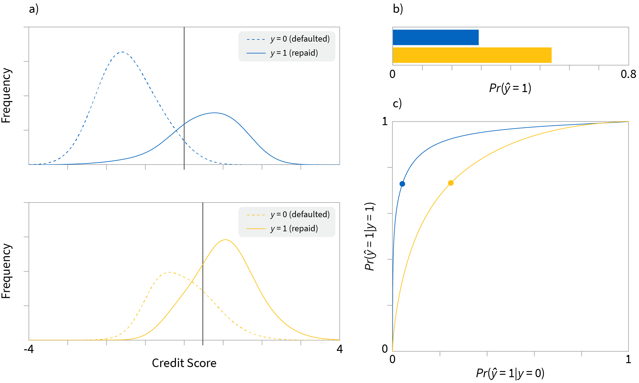
Figure 4. Equal opportunity. a) We choose thresholds so that that c) the true positive rate $Pr(\hat{y}=1|y=1)$ is the same between the two populations; the vertical position of the points on the ROC curve match. This means that the same proportion of blue and yellow groups pay back their loans. b) It has the disadvantage that different numbers of loans are given to each population.
Trade-offs
We have seen that there is no straightforward way to choose thresholds on an existing classifier for different populations, so that all definitions of fairness are satisfied. Now we’ll investigate a different approach that aims to make the classification performance more similar for the two models.
The ROC curves show that accuracy is higher in predicting whether the blue population will repay the loan as opposed to the yellow group (i.e. the blue ROC curve is everywhere higher than the yellow one). What if we try to reduce the accuracy for the blue population so that this more nearly matches? One way to do this is to add noise to the credit score for the blue population (figure 5). As we add increasing amounts of noise the blue ROC curve moves towards the positive diagonal and at some point will cross the yellow ROC curve. Now equality of odds can be achieved.

Figure 5. Adding noise to improve fairness. a-c) We progressively add noise to the blue credit scores, causing the distributions to become flatter and overlap more. e) As we add noise, the blue ROC curve moves towards the positive diagonal and at some point must intersect the yellow ROC curve, meaning that equality of odds can be achieved.
Unfortunately, this approach has two unattractive features. First, we now make worse decisions for the blue population; it is a general feature of most remedial approaches that there is a trade off between accuracy and fairness (Kamiran & Calders 2012; Corbett-Davies et al. 2017). Second, adding noise violates individual fairness. Two identical members of the blue population may have different noise values added to the scores, resulting in different decisions on their loans.
Bias mitigation algorithms
The conclusion of the worked loan example is that it is very hard to remove bias once the classifier has already been trained, even for very simple cases. For further information, the reader is invited to consult Kamiran & Calders (2012), Hardt et al. (2016), Menon & Williamson (2017) and Pleiss et al. (2017).
| Post-Processing | In-Processing | Pre-Processing | Data Collection |
| • Change thresholds • Trade off accuracy for fairness | • Adversarial training • Regularize for fairness • Constrain to be fair | • Modify labels • Modify input data • Modify label/data pairs • Weight label/data pairs | • Identify lack of examples or variates and collect |
Thankfully, there are approaches to deal with bias at all stages of the data collection, preprocessing, and training pipeline (figure 6). In this section we consider some of these methods. In the ensuing discussion, we’ll assume that the true behaviour of the different populations is the same. Hence, we are interested in making sure that the predictions of our system do not differ for each population.
Pre-processing approaches
A straightforward approach to eliminating bias from datasets would be to remove the protected attribute and other elements of the data that are suspected to contain related information. Unfortunately, such suppression rarely suffices. There are often subtle correlations in the data that mean that the protected attribute can be reconstructed. For example, we might remove race, but retain information about the subject’s address, which could be strongly correlated with the race.
The degree to which there are dependencies between the data $\mathbf{x}$ and the protected attribute $p$ can be measured using the mutual information
\begin{equation}
\mbox{LP} = \sum_{\mathbf{x},p} Pr(\mathbf{x},p) \log\left[\frac{Pr(\mathbf{x},p)}{Pr(\mathbf{x})Pr(p)}\right], \tag{2.6}
\end{equation}
which is known as the latent prejudice (Kamishima et al. 2011). As this measure increases, the protected attribute becomes more predictable from the data. Indeed, Feldman et al. (2015) and Menon & Williamson (2017) have shown that the predictability of the protected attribute puts mathematical bounds on the potential discrimination of a classifier.
We’ll now discuss four approaches for removing bias by manipulating the dataset. Respectively, these modify the labels $y$, the observed data $\mathbf{x}$, the data/label pairs $\{{\mathbf{x},y\}}$, and the weighting of these pairs.
Manipulating labels
Kamiran & Calders (2012) proposed changing some of the training labels which they term massaging the data. They compute a classifier on the original dataset and find examples close to the decision surface. They then swap the labels in such a way that a positive outcome for the disadvantaged group is more likely and re-train. This is a heuristic approach that empirically improves fairness at the cost of accuracy.
Manipulating observed data
Feldman et al. (2015) proposed manipulating individual data dimensions $x$ in a way that depends on the protected attribute $p$. They align the cumulative distributions $F_{0}[x]$ and $F_{1}[x]$ for feature $x$ when the protected attribute $p$ is 0 and 1 respectively to a median cumulative distribution $F_{m}[x]$. This is similar to standardising test scores across different high schools (figure 7) and is termed disparate impact removal. This approach has the disadvantage that it treats each input variable $x\in\mathbf{x}$ separately and ignores their interactions.
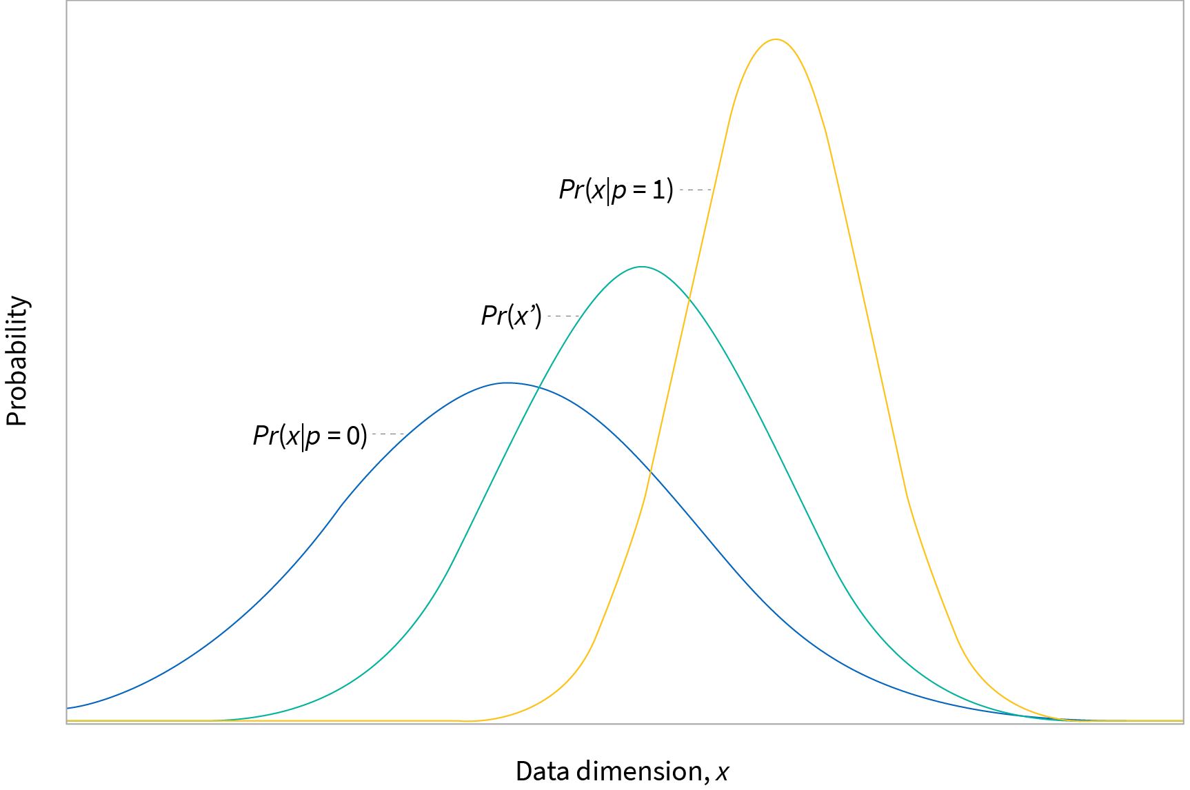
Figure 7. Disparate impact removal. Blue and yellow curves represent a single input data dimension $x$ for blue population $p=0$ and yellow population $p=1$. Feldman et al. (2015) propose to de-bias the dataset by mapping each to a median distribution (green curve) using cumulative distribution functions.
Manipulating labels and data
Calmon et al. (2017) learn a randomized transformation $Pr(\mathbf{x}^{\prime}, y^{\prime}|\mathbf{x},y,p)$ that transforms data pairs $\{\mathbf{x}, y\}$ to new data values $\{\mathbf{x}^{\prime}, y^{\prime}\}$ in a way that depends explicitly on the protected attribute $p$. They formulate this as an optimization problem in which they minimize the change in data utility, subject to limits on the prejudice and distortion of the original values. They show that this optimization problem may be convex in certain conditions.
Unlike disparate impact removal, this takes into account interactions between all of the data dimensions. However, the randomized transformation is formulated as a probability table, so this is only suitable for datasets with small numbers of discrete input and output variables. The randomized transformation, which must also be applied to test data, also violates individual fairness.
Reweighting data pairs
Kamiran & Calders (2012) propose to re-weight the $\{\mathbf{x}, \mathbf{y}\}$ tuples in the training dataset so that cases where the protected attribute $p$ predicts that the disadvantaged group will get a positive outcome are more highly weighted. They then train a classifier that makes use of these weights in its cost function. Alternately, they propose re-sampling the training data according to these weights and using a standard classifier.
In-processing algorithms
In the previous section, we introduced the latent prejudice measure based on the mutual information between the data $\mathbf{x}$ and the protected attribute $p$. Similarly, we can measure the dependence between the labels $y$ and the protected attribute $p$:
\begin{equation}
\mbox{IP} = \sum_{y,p} Pr(y,p) \log\left[\frac{Pr(y,p)}{Pr(y)Pr(p)}\right]. \tag{2.7}
\end{equation}
This is known as the indirect prejudice (Kamishima et al. 2011). Intuitively, if there is no way to predict the labels from the protected attribute and vice-versa then there is no scope for bias.
One approach to removing bias during training is to explicitly remove this dependency using adversarial learning. Other approaches to removing bias include penalizing the mutual information using regularization, fitting the model under the constraint that it is not biased. We’ll briefly discuss each in turn.
Adversarial de-biasing
Adversarial-debiasing (Beutel et al. 2017; Zhang et al. 2018) reduces evidence of protected attributes in predictions by trying to simultaneously fool a second classifier that tries to guess the protected attribute $p$. Beutel et al. (2017) force both classifiers to use a shared representation and so minimizing the performance of the adversarial classifier means removing all information about the protected attribute from this representation (figure 8).
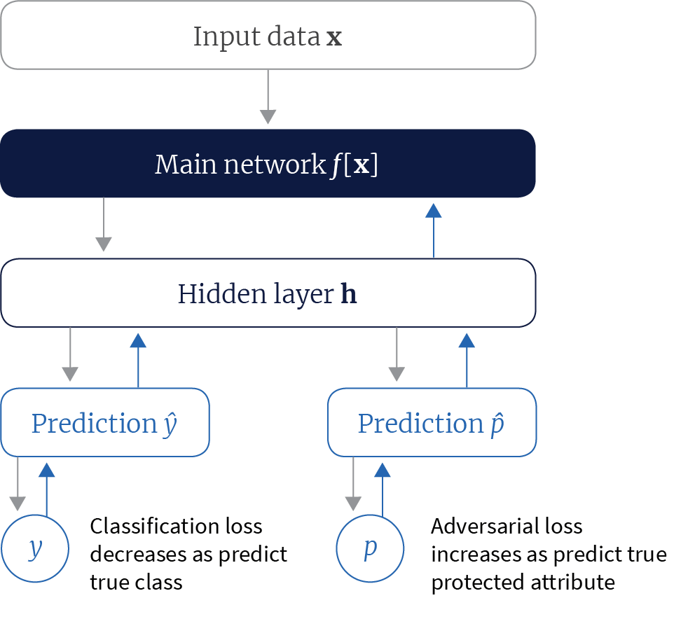
Figure 8. Adversarial learning for fairness. Beutel et al. (2017) learned a representation for classification that was also used to predict the protected attribute. The system was trained in an adversarial manner, encouraging good performance by the system but punishing correct classification of the protected attribute. In this way a representation that does not contain information about the protected attribute is learned.
Zhang et al. (2018) use the adversarial component to predict $p$ from (i) the final classification logits $f[\mathbf{x}]$ (to ensure demographic parity), (ii) the classification logits $f[\mathbf{x}]$ and the true class $y$ (to ensure equality of odds), or (iii) the final classification logits and the true result for just one class (to ensure equality of opportunity).
Prejudice removal by regularization
Kamishima et al. (2011) proposed adding an extra regularization condition to the output of logistic regression classifier that tried to minimize the mutual information between the protected attribute and the prediction $\hat{y}$. They first re-arranged the indirect prejudice expression using the definition of conditional probability to get
\begin{eqnarray}
\mbox{PI} &=& \sum_{y,p} Pr(y|\mathbf{x},p) \log\left[\frac{Pr(y,p)}{Pr(y)Pr(p)}\right]\nonumber\\
&=& \sum_{y,p} Pr(y|\mathbf{x},p) \log\left[\frac{Pr(y|p)}{Pr(y)}\right]. \tag{2.8}
\end{eqnarray}
Then, they formulate a regularization loss based on the expectation of this over the data set:
\begin{equation}
\mbox{L}_{reg} = \sum_{i}\sum_{\hat{y},p}
Pr(\hat{y}_{i}|\mathbf{x}_{i},p_{i})\log\left[\frac{Pr(\hat{y}_{i}|p_{i})}{Pr(\hat{y}_{i})}\right] \tag{2.9}
\end{equation}
where $i$ indexes the data examples, which they add to the main training loss.
Fairness constraints
Zafar et al. (2015) formulated unfairness in terms of the covariance between the protected attribute $\{p_{i}\}_{i=1}^{I}$ and the signed distances $\{d[\mathbf{x}_{i},\boldsymbol\theta]\}_{i=1}^{I}$ of the associated feature vectors $\{\mathbf{x}_{i}\}_{i=1}^{I}$ from the decision boundary, where $\boldsymbol\theta$ denotes the model parameters. Let $\overline{p}$ represent the mean value of the protected attribute. They then minimize the main loss function such that the covariance remains within some threshold $t$.
\begin{equation}
\begin{aligned}
& \underset{\boldsymbol\theta}{\text{minimize}}
& & L[\boldsymbol\theta] \\
& \text{subject to}
& & \frac{1}{I}\sum_{i=1}^{I}(p_{i}-\overline{p})d[\mathbf{x}{i},\boldsymbol\theta] \leq t\\ & & & \frac{1}{I}\sum{i=1}^{I}(p_{i}-\overline{p})d[\mathbf{x}_{i},\boldsymbol\theta] \geq -t
\end{aligned} \tag{2.10}
\end{equation}
This constrained optimization problem can also be written as a regularized optimization problem in which the fairness constraints are moved to the objective and the corresponding Lagrange multipliers act as regularizers. Zafar et al. (2015) also introduced a second formulation where they maximize fairness under accuracy constraints.
Other approaches
Zemel et al. (2013) presented a method that maps data to an intermediate space in a way that depends on the protected attribute and obfuscates information about that attribute. Since this mapping is learnt during training, this method could considered either a pre-processing approach or an in-processing algorithm.
Chen et al. (2018) argue that a trade off between fairness and accuracy may not be acceptable and that these challenges should be addressed through data collection. They aim to diagnose unfairness induced by inadequate data and unmeasured predictive variables and prescribe data collection approaches to remedy these problems.
Summary and further resources
In this tutorial, we’ve discussed what it means for a classifier to be fair, how to quantify the degree of bias in a dataset and methods to remedy unfairness at all stages in the pipeline. An empirical analysis of fairness-based interventions is presented in Friedler et al. (2019). There are a large number of toolkits available to help evaluate fairness, the most comprehensive of which is AI Fairness 360.
This tutorial has been limited to a discussion of supervised learning algorithms, but there is also an orthogonal literature on bias in NLP embeddings (e.g. Zhao et al. 2019).
Work with Us!
Impressed by the work of the team? RBC Borealis is looking to hire for various roles across different teams. Visit our career page now and discover opportunities to join similar impactful projects!
Careers at RBC Borealis