In the first part of this tutorial we introduced the Boolean satisfiability problem and discussed applications. In the second part, we developed algorithms based on tree search for solving satisfiability problems. This third, and final part is divided into two sections, each of which is self-contained. First, we consider a completely different approach to solving satisfiability problems which is based on factor graphs. Second, we will discuss methods that allow us to apply the SAT machinery to problems with continuous variables.
Satisfiability as a function of problem size
To motivate the factor graph approach to SAT solving, we will first consider how the difficulty of satisfiability scales with the problem size. If we are given a random formula with $V$ variables, and $C$ clauses, each of clause length $K$, how likely is it that there is a configuration of variables that will return $\text{SAT}$? Considering each of these parameters in turn:
- As the number of clauses $C$ increases, satisfiability becomes less probable for a fixed number of variables; each clause adds a constraint to the solution (figure 1).
- As the clause length $K$ increases, satisfiability becomes more probable given a fixed number of clauses. Since the terms within a clause are connected by a logical $\text{OR}$ operator, only one needs to be $\text{true}$ for the whole clause to be $\text{true}$ and so longer clause lengths are easier to satisfy (figure 2).
- As the number of variables increases (keeping the number of clauses and the clause lengths the same), then the problem becomes easier as there are less constraints per variable.

Figure 1. Satisfiability as a function of number of clauses. Consider satisfiability problems with $V=5$ variables and clause length $K=3$. For this configuration there are 80 distinct possible clauses. We construct problems with by randomly selecting $C$ of these clauses without repetition. Since there are only 5 variables, there are 32 possible solutions and for each problem we can search them exhaustively to see if one satisfies an expression. The plot shows the probability that the expression can be satisfied as a function of the number of clauses. As we might expect, expression with very few constraints are always satisfiable, whereas expressions with many constraints are never satisfiable. Adapted from Knuth (2015).

Figure 2. Satisfiability as a function of clause length for random problems constructed as in figure 1. As the clause length increases, the probability that the expression can be satisfied for a fixed number of clauses increases; looking at it another way, as clause length increases, we can add more clauses on average before the expression cannot be satisfied. Adapted from Knuth (2015).
Clause:variable ratio and phase change
The clause:variable ratio $C/V$ is a critical factor in determining the probability that an expression will be satisfiable. Consider increasing the number of clauses and the number of variables, but keeping this ratio constant. For very large numbers of clauses and variables, there is a distinct threshold below which almost all problems are satisfiable and above which almost all problems are not satisfiable. This is known as a phase change.
For the 2-SAT problem, the phase change can be proven to occur at a clause:variable ratio of $C/V = 1.0$. For 3-SAT it has been empirically observed at $C/V \approx 4.27$ (figure 3). This is not mathematically proven although lower and upper bounds of 3.52 and 4.49 respectively have been proved.

Figure 3. Satisfiability as a function of clause:variable ratio for 3-SAT. Most 3-SAT problems with a clause:variable ratio of less than 4.27 are satisfiable, whereas most problems with a ratio of greater than this are not satisfiable. As the ratio is kept constant but the absolute number of variables $V$ and clauses $C$ increases, this behaviour becomes more pronounced and eventually takes the form of a step function. Adapted from Knuth (2015).
These results should be interpreted with some caution. This analysis concerns randomly generated expressions. For real problems, the clauses are not chosen randomly but relate to the structure of the underlying problem. Nonetheless, they provide some insight into the difficulty of SAT problems as a function of their constituent parts.
Energy barriers and algorithm choice
The clause:variable ratio is also important in determining the type of algorithms that we should apply to SAT problems. As we approach the phase change threshold, satisfying solutions are thought to be sparse and separated by large energy barriers (figure 4). In this regime, the search-based methods that we described in part II of this tutorial do not necessarily work well. However, by re-framing the problem in terms of factor graphs, we can develop algorithms that function well in this part of the space.

Figure 4. SAT problem solution space as a function of the clause:variable ratio. Black dots represent valid solutions and blue dots invalid ones. a) At low clause:variable ratios, there are many solutions and they are mostly connected to one another in terms of Hamming distance. In this regime, any SAT solver is appropriate. b) As the clause:variable ratio increases the solutions become more infrequent and occur in separate clusters separated by infeasible solutions. In this regime, the survey propagation algorithm (an extension of belief propagation) is the best option. c) Above a certain clause to ratio threshold there are very few or no solutions. Adapted from Maneva et al. (2008).
In the following section we’ll discuss the relation between SAT solving and factor graphs and show that satisfiability can be established using belief propagation. We’ll also introduce the survey propagation algorithm, which is the method of choice for very difficult SAT problems that are expressed in terms of factor graphs.
Factor graph representation of SAT
Up until this point, we have treated SAT solving as a search for literals that satisfy a formula. A slightly different viewpoint is to consider taking the logical $\text{OR}$ of $2^{V}$ copies the SAT formula where each copy contains one of the possible solution sets of the literals. If this compound statement evaluates to $\text{true}$ then it means that at least one of the possible solutions evaluates to $\text{true}$ and so the formula is satisfiable.
To express this idea mathematically, let’s denote the $c^{th}$ clause as a function $\mbox{f}[\mathbf{x}_{\mathcal{S}_{c}}]$ of a subset $\mathcal{S}_{c}$ of the variables $\{x_{i}\}_{i=1}^{I}$ that returns $\text{true}$ or $\text{false}$. The SAT formula now looks like
\begin{equation} \phi := \mbox{f}[\mathbf{x}_{\mathcal{S}_{1}}] \land \mbox{f}[\mathbf{x}_{\mathcal{S}_{2}}] \land \ldots \land \mbox{f}[\mathbf{x}_{\mathcal{S}_{C}}] \tag{1}\end{equation}
and we can express the logical $\text{OR}$ing of all $2^{V}$ combinations of variables as:
\begin{equation}\phi’:= \bigvee_{x_{1}}\left[\bigvee_{x_{2}}\left[\ldots \bigvee_{x_{V}}\left[ \mbox{f}[\mathbf{x}_{\mathcal{S}_{1}}] \land \mbox{f}[\mathbf{x}_{\mathcal{S}_{2}}] \land \ldots \land \mbox{f}[\mathbf{x}_{\mathcal{S}_{C}}]\right]\right]\right] \tag{2}\end{equation}
where the notation $\bigvee_{x_{1}}[\boldsymbol\phi] = (\phi\land x_{1})\lor (\phi\land \overline{x_{1}})$ logically $\text{OR}$s together two copies of the expression where we have set $x_{1}$ to $\text{true}$ and $\text{false}$ respectively.
Of course, this is not very practical, because the resulting expression will have an $2^{V}$ terms. However, this form elucidates a connection with graphical models. Instead of considering the functions returning $\text{true}$ or $\text{false}$, let’s modify them so that they return the real numbers $1$ when $\text{true}$ and $0$ when $\text{false}$. Now we can write:
\begin{eqnarray}\phi’&:=& \max_{x_{1}}\left[\max_{x_{2}}\left[\ldots \max_{x_{V}}\left[ \mbox{f}[\mathbf{x}_{\mathcal{S}_{1}}] \cdot \mbox{f}[\mathbf{x}_{\mathcal{S}_{2}}] \cdot \ldots \cdot \mbox{f}[\mathbf{x}_{\mathcal{S}_{C}}]\right]\right]\right] \nonumber \\&=&\max_{x_{1},x_{2}\ldots x_{V}}\left[\prod_{c=1}^{C} \mbox{f}[\mathbf{x}_{\mathcal{S}_{c}}]\right] \tag{3}\end{eqnarray}
where we have replaced the logical $\text{AND}$s by multiplication operations and the $\bigvee_{x}$ operations by a maximization over the two possible binary values of $x$. In a valid solution each function (clause) will return 1 and hence so will their product. In an invalid solution, one of the functions will return 0 and hence the product will be zero. It follows that if the maximum possible output of this product is 1, then at least one solution must be true and the formula is satisfiable.
SAT as maximum-likelihood in a probabilistic model
We can now view the SAT problem in terms of finding the maximum likelihood solution in an undirected graphical model with cliques $\mathcal{S}_{c}$:
\begin{equation}\label{eq:SAT_as_Prob} Pr(\mathbf{x}) = \frac{1}{Z}\prod_{c=1}^{C}\mbox{f}[\mathbf{x}_{\mathcal{S}_{c}}] \tag{4}\end{equation}
where the normalizing constant $Z$ is known as the partition function. Since the un-normalized function yields $1$ for each valid solution and $0$ for each invalid solution, the partition function counts the number of valid solutions.
If maximizing the unnormalized distribution with respect to the binary variables $\{x_{i}\}_{i=1}^{V}$ yields $1$ then all the terms are simultaneously satisfiable and we have found a solution. As a concrete example, consider the formula:
\begin{equation} \phi:= (x_{1}\lor \overline{x}_{2}) \land (\overline{x}_{1} \lor x_{3}) \land ({x}_{2} \lor x_{3} \lor \overline{x}_{4}) \land (\overline{x}_{3} \land x_{5}) \land(\overline{x}_{3}\lor x_{4}\lor x_{5}). \tag{5}\end{equation}
Solving the satisfiability problem for this formula is equivalent to maximizing the probability in the factor model in figure 5 with respect to the discrete variables $x_{i}$.

Figure 5. SAT problems as factor models. a) Clauses from a SAT problem in conjunctive normal form. b) Factor graph representation of this formula. Each clause is represented by a factor. By convention we draw solid lines when the literal $x_{i}$ contributes to the factor and dashed lines when the literal $\overline{x}_{i}$ contributes to the factor.
Max-product algorithms
Inference in factor graphs can be tackled using belief propagation. If the factor graph takes the form of a chain or a tree (i.e. has no loops) then we can find the maximum likelihood solution exactly in polynomial time using the max-product algorithm. However, this is rarely the case and so we must rely on loopy belief propagation, which is not guaranteed to find the global maximum, but often finds a good solution in practice. Both these algorithms involve repeatedly passing messages between neighboring variables on the graph.
Note that this method can also be used for Max-SAT problems. Here, the assumption is that there is no satisfying solution and we aim to find the maximum number of clauses that can be simultaneously satisfied. It can also be trivially adapted to the weighted Max-SAT problem (in which there is a different penalty for each clause being left unsatisfied).
From max-product to sum-product
Since we have expressed the SAT problem as a probability distribution (equation 4), we could also consider computing the marginals of this distribution. The marginal distribution of a variable $x_{i}$ indicates the proportion of solutions in which $x_{i}$ evaluates to $\text{true}$ and $\text{false}$. If this distribution indicates that one or the other solution is almost certain, then we could just fix this value and hence reduce the complexity of the problem. This process is known as decimation. One approach to establishing satisfiability is hence to alternate between decimating and then finding the marginals again in the new simpler problem.
The marginal distributions for all of the variables can be computed at the same time using the sum-product algorithm. Once more, if the graph structure is a chain or tree then this can be done both exactly and efficiently. However, for practical problems this is rarely the case and we must resort again to a loopy belief propagation algorithm. This provides an approximate estimate of the marginal distributions, which may in some circumstances be good enough to choose variables to decimate.
The sum-product algorithm has another fringe benefit in that it also computes the partition function (or an estimate thereof in the loopy case). Hence, we can use this approach to solve the model counting problem (#SAT problem) in which we want to know the total number of valid solutions.
Survey propagation
A disadvantage of the max-product and sum-product approaches is that they do not fully explore the solution space. Their approach is analogous to gradient methods in optimization in that they converge on a local maximum, but may miss the best overall solution. This is particularly problematic when the clause:variable ratio approaches the phase change threshold; recall that here the satisfying solutions are thought to be sparse and separated by large energy barriers.
One approach to finding satisfying assignments in this regime is to use survey propagation. This can be thought of a meta-belief propagation algorithm. In the sum-product algorithm, the messages passed provide information about the distribution over variable assignments. In survey propagation, the messages passed provide information about the messages in the belief propagation sum-product algorithm. In a sense, survey propagation is considering the full family of possible sum-product solutions simultaneously and so is less prone to getting stuck in local minima. It also has a superior estimate of the true marginals with which it can better inform the decimation process. As before, survey propagation is alternated with a decimation process as we gradually fix variables and simplify the problem.
Conclusion
This concludes the discussion of SAT algorithms that we started in part II of this tutorial. To summarize, SAT problems get harder as the clause:variable ratio approaches the phase transition value and different methods are required. Hence we re-formulated the satisfiability problem in terms of maximum likelihood on a factor graph model. We then discussed a series of methods based on max-product, sum-product, and survey propagation algorithms. These approaches also have the fringe benefit of being applicable to the Max-SAT, weighted Max-SAT and model counting problems.
In the next two sections, we change tack completely and discuss the extension of SAT method to non-binary variables.
Conversion from non-binary variables
The reader may have some lingering doubt as to the utility of an optimization method that can only work with binary variables. However, the machinery of SAT solvers can be leveraged to use integer or floating point variables. We’ll present two approaches. In this section, we consider converting problems that are not naturally binary into a binary form and using the standard SAT machinery to solve them. In the following section, we consider generalizing the SAT framework to allow continuous variables using satisfiability modulo theory solvers.
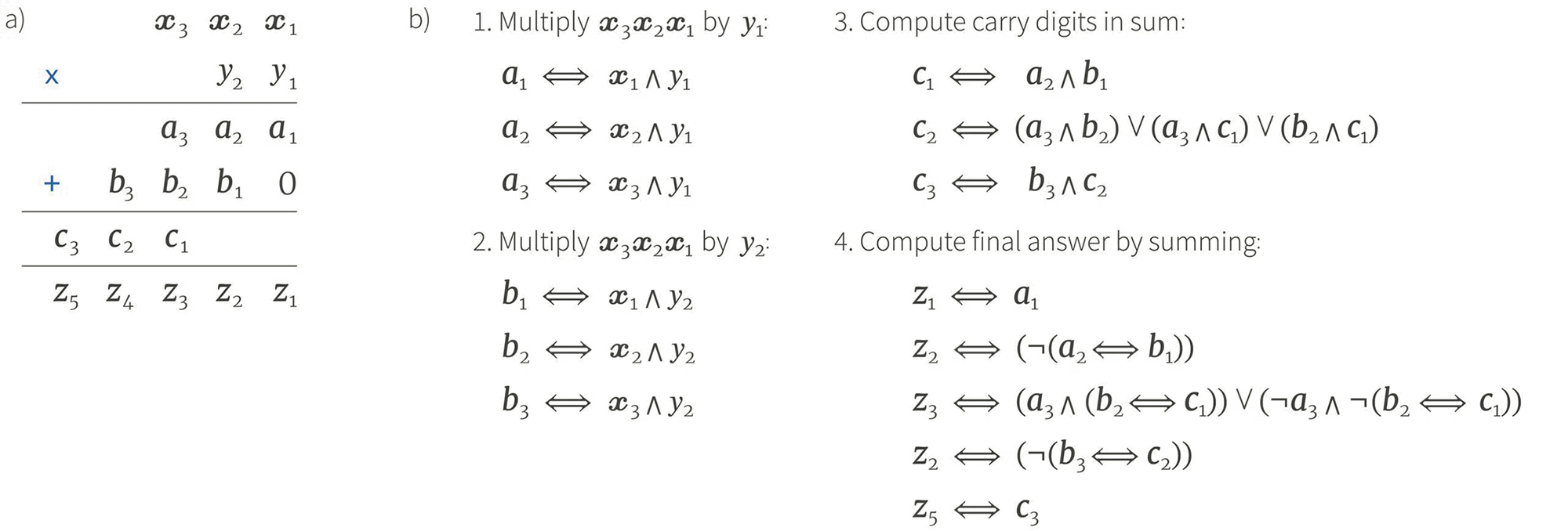
The former approach is very simple. We convert the non-binary variables to a binary form and express the constraints that tie them together as a series of binary relations. To help understand this, we adapt an example from Knuth (2015). Consider the problem of factoring a known integer $Z$: given this integer we aim to return two other integers $X$ and $Y$ that multiply together to give $Z$ or return $\text{UNSAT}$ if this is not possible.
First we express the variables in binary form so that, for example $X=x_{3}x_{2}x_{1}$ where $x_{3}$ represents the most significant digit and $x_{1}$ the least, so that the decimal number 5 would be represented as $x_{3}x_{2}x_{1} = 101$. Then we note that to multiply two binary numbers we can use a variation of the method taught in schools (figure 6a). The sub-operations needed to perform this method can all be expressed in terms of logical relations. When we run a SAT solver on this problem, it will either succeed and return possible values for $X$ and $Y$ in binary form, or it will return $\text{UNSAT}$. In a more practical system we might want to add a further condition that neither $X$ nor $Y$ are 1 which gives a trivial factorization.

Figure 6. Factorizing an integer $Z$ using a SAT solver. We seek values for $X = x_{3},x_{2},x_{1}$ and $Y= y_{2},y_{1}$ so that when these numbers are multiplied together, we get some predetermined number $Z = z_{5}z_{4}z_{3}z_{2}z_{1}$, where all of these integers are expressed in binary form. a) The multiplication operation can be done using the method taught in school, but using binary variables. b) The sub operations (two multiplications by a single digit, and adding the results taking account of carry digits) can all be expressed as logical relations.
This type of approach is not limited to working with integers. We could similarly represent real-numbers in binary form up to some pre-specified precision. However, one disadvantage of the approach is that it requires a lot of clauses to represent simple relationships between the non-binary variables. In the following section, we discuss SMT solvers which can work directly with integers or floating point numbers without converting them to a binary form.
SMT solvers
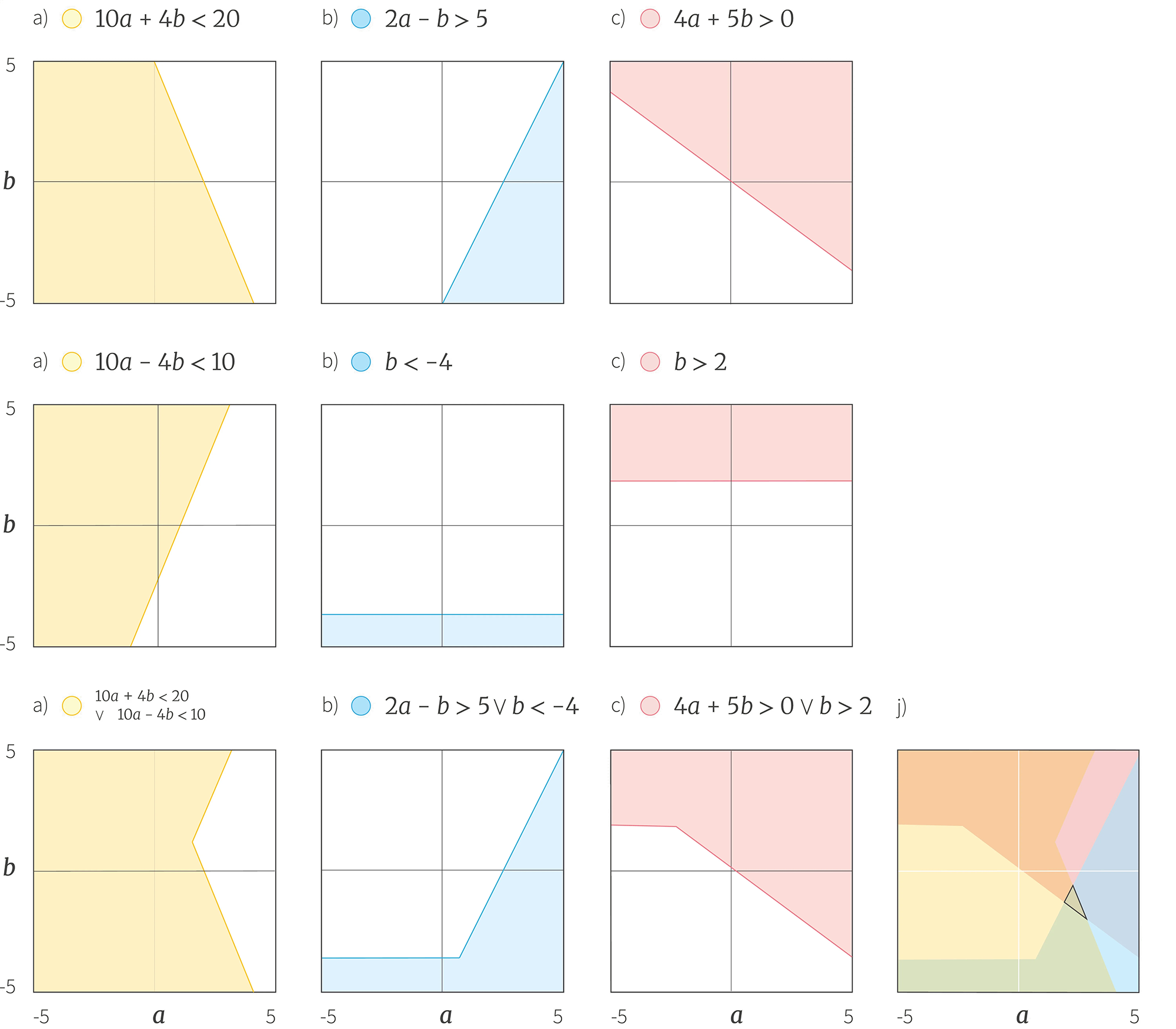
Satisfiability modulo theories (SMT) problems generalize the SAT problem so that the binary variables are replaced by predicates that are taken from a particular family. A predicate is a binary valued function of the non-binary variables. One common example of a family of predicates is linear inequalities such as $a + b > 0$. The associated SMT problem might consider expressions in conjunctive normal form like:
\begin{eqnarray}\label{eq:SMTExample} \phi&:=& \left((10a+4b<20) \lor (10a-4b<10) \right) \land \nonumber \\ &&\hspace{1cm}\left((2a-b>5) \lor (b<-4) \right) \land \left( (4a+5b>0)\lor (b>2)\right) \tag{6}\end{eqnarray}
where are asking the question of whether there is any combination of continuous values $a, b$ that make this expression evaluate to $\text{true}$ (figure 7).

Figure 7. Graphical exploration of SMT Example. a-f) Graphical representation of the six linear equalities in equation 6. g) The first clause takes the logical $\text{OR}$ of two of the inequalities and this means that the union of their valid regions is now valid. h) Similarly the second clause takes the logical $\text{OR}$ of another two of the inequalities. i) The third clause takes the logical $\text{OR}$ of the remaining two inequalities. j) To test if the conjunction of the three clauses is $\text{true}$, we superimpose the regions defined by each clause and observe that there is a small triangular region where they all overlap and hence this formula is satisfiable.
Theory solvers
To solve a problem of this type, we need an efficient algorithm that tests whether a conjunction (logical $\text{AND}$) of the predicates are satisfiable. This is known as a theory solver. For this example, the theory solver tests if a set of linear inequalities are simultaneously feasible. Luckily, there is a well established method to do this, which is the first step of the Simplex algorithm for linear programming. For the purposes of the remaining discussion, we’ll treat the theory solver as a black box that returns $\text{true}$ if a set of inequalities are simultaneously feasible and $\text{false}$ otherwise.
Lazy SMT solving
In the lazy approach to SMT solving, we integrate the theory solver into the standard tree-search SAT solver approach. Continuing our worked example, we associate a binary literal $x_{i}$ with each of the six inequalities in equation 6 so the formula now looks like:
\begin{equation}\phi:= (x_{1} \lor x_{2}) \land (x_{3}\lor x_{4}) \land (x_{5}\lor x_{6}) \tag{7}\end{equation}
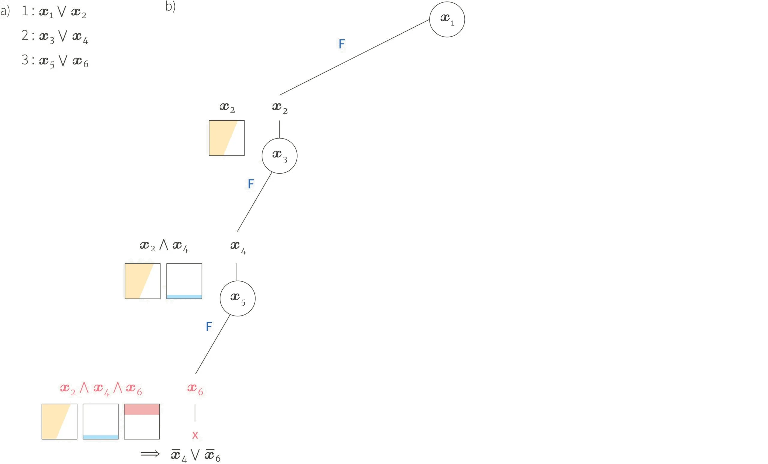
Then we proceed with the DPLL tree search (figure 8). As we search through the tree, we set $x_{1}$ to $\text{false}$, which means that by unit resolution $x_{2}$ must be $\text{true}$ for the first clause to be valid. Then we set $x_{3}$ to $\text{false}$ which means that $x_{4}$ must be $\text{true}$. At this point we have established that $x_{2}$ and $x_{4}$ must both be valid and so we use our theory solver to test if $x_{2}\land x_{4}$ is possible. It turns out that it is, and so we continue. We set $x_{5}$ to $\text{false}$ and this implies that $x_{6}$ must be $\text{true}$ and so we now use the theory solver to test if $x_{2}\land x_{4} \land x_{6}$ is feasible. These three inequalities cannot be simultaneously satisfied and so the theory solver returns $\text{false}$.

Figure 8. SMT lazy approach. a) Clauses from the formula in conjunctive normal form. b) We apply the DPLL algorithm as usual. Starting at the root node, we set $x_{1}$ to $\text{false}$ which implies by clause 1 that $x_{2}$ is $\text{true}$. Then we set $x_{3}$ to $\text{false}$ which implies that $x_{4}$ must be $\text{true}$. Now we use the theory solver to test if $x_{2}\land x_{4}$ is feasible. We can see that this is the case because the yellow and blue areas overlap. So we continue through the tree by setting $x_{5}$ to $\text{false}$ which implies that $x_{6}$ must be $\text{true}$. We now use the theory solver again to test if $x_{2}\land x_{4}\land x_{6}$ is feasible. We can see that this is not the case because there is no place where the yellow, blue and red regions intersect, and more specifically, $x_{4}$ and $x_{6}$ cannot be simultaneously satisfied. This generates the new clause $\overline{x}{4}\lor\overline{x}{6}$ which we add to the formula.
Recycling clauses
In principle, we could continue in this way exploring the tree exhaustively until we either find a solution that is $\text{SAT}$ or we terminate and return $\text{UNSAT}$. However, as in conflict driven clause learning, we can make the solution considerably more efficient by adding a new term reflecting what we have learnt from the theory solver. In this case, we find that $x_2 \land x_{4} \land x_{6}$ cannot be $\text{true}$. Analyzing this more carefully, it turns out that this is because $x_{4}$ and $x_{6}$ are incompatible so we add the term $\overline{x}_{4} \lor \overline{x}_{6}$ to give the new formula.
\begin{equation}\phi’:= (x_{1} \lor x_{2}) \land (x_{3}\lor x_{4}) \land (x_{5}\lor x_{6}) \land (\overline{x}_{4} \lor \overline{x}_{6}). \tag{8}\end{equation}
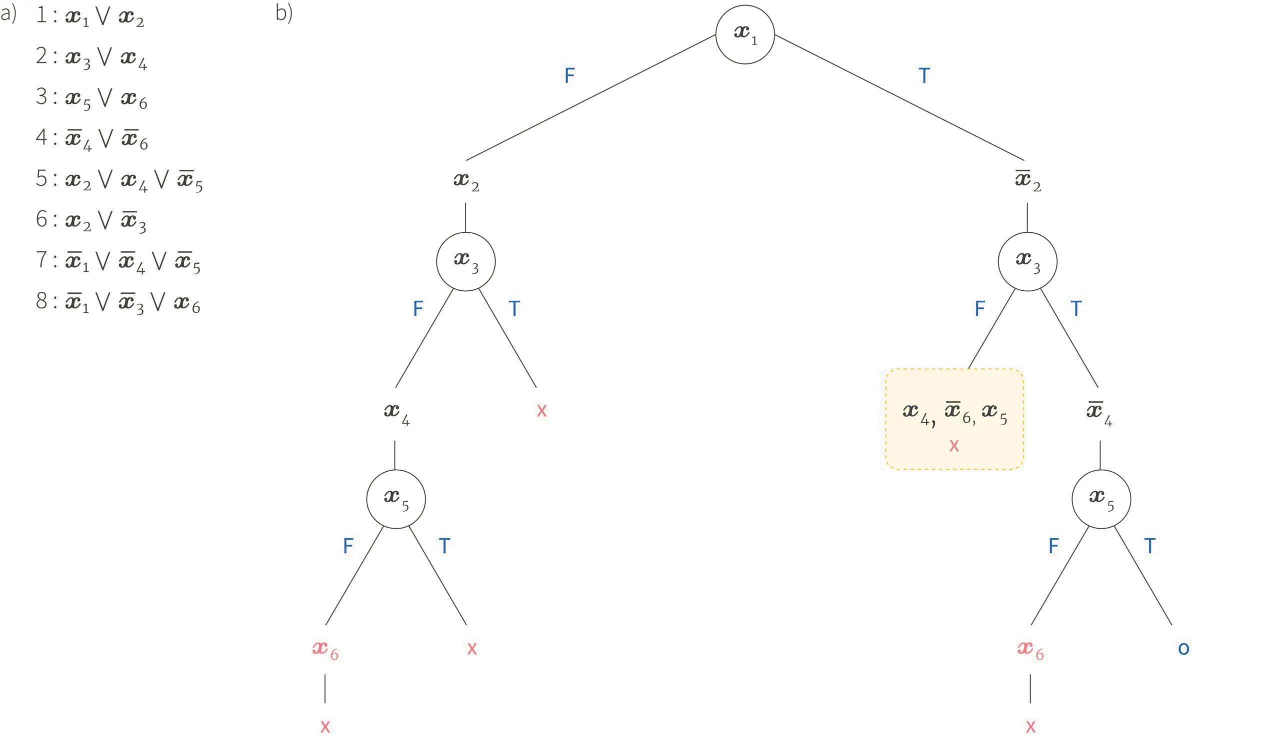
Now we continue the search using the same procedure, but with the extended formula . Each time that the theory solver returns that a subset of the constraints are incompatible, we add this to the SAT formula. We continue this until we either exhaust the possibilities or find the solution. The full tree is illustrated in figure 9 and it finds the solution $x_{1}\land x_{3}\land x_{5}$ which visual inspection of figure 7 indicates are indeed the three regions that have a valid intersection.
Note that at the tree node in the yellow rectangle in figure 9, we eliminate an entire fork of the tree based on the SAT solver as a result of adding the clauses. In a full-scale problem, this means that we can eliminate many parts of the search space using the SAT solver and hence reduce the number of times that we need to call the more expensive theory solver.

Figure 9. SMT lazy approach continued. a) The full set of clauses generated at the end of the search. b) The full tree at the end of the search. The tree node in the yellow rectangle is particularly interesting. When we reach this point, we have the first six clauses. When we choose $\overline{x}_{3}$ at the node above, this sets off a chain of unit resolution. First, $\overline{x}_{3}$ implies that $x_{4}$ must be $\text{true}$ by clause $2$. Then $\overline{x}_{6}$ must be $\text{true}$ by clause 4, and finally $x_{5}$ must be $\text{true}$ by clause 3. In this way, we eliminate a fork of the tree based on the SAT solver alone without having to use the more expensive theory solver.
In conclusion, the lazy approach to SMT solving can be employed as long as we have an efficient theory solver that can evaluate whether an arbitrary conjunction of predicates are $\text{true}$. The SAT solver and the theory solver work in conjunction. Cases where the theory solver failed are added back to the tree which effectively prunes the search procedure and reduces the number of times that we have to use the theory solver in the future.
Conclusion and further reading
This series of tutorials has introduced the basics of the satisfiability problem and the algorithms that are used to solve it. It is our opinion that this sophisticated machinery is under-used in AI and that there is considerable scope for combining it with more mainstream machine learning techniques.
For further information about SAT solving including the DPLL and CDCL algorithms, consult the Handbook of Satisfiability. A second useful resource is Donald Knuth’s Facsicle 6. For further reading about random SAT problems and the phase change, the relation between SAT and factor graphs and the survey propagation algorithm, consult Information, physics, and computation. For an extremely comprehensive list of applications of satisfiability, consult SAT/SMT by example. If you want to practically use a SAT solver, this tutorial will help you get started.
Work with Us!
Impressed by the work of the team? RBC Borealis is looking to hire for various roles across different teams. Visit our career page now and discover opportunities to join similar impactful projects!
Careers at RBC Borealis