In part I of this three part series on transformers, we introduced self-attention and the transformer architecture, and we discussed how the transformer is used in NLP. In this blog, we’ll focus on two families of modifications that address limitations of the basic architecture and draw connections between transformers and other models. This blog will be suitable for someone who knows how transformers work, and wants to know more about subsequent developments.
In the first section, we’ll discuss position embeddings. The transformer operates on unordered sets of embeddings, but often we are processing ordered sequences (e.g., words in NLP). We will describe the ways that the architecture has been adapted to take into account the position of each element in the sequence. In the second section, we’ll discuss efficiency. The attention computation grows quadratically with the sequence length and in practice this limits the maximum length we can use. We’ll describe work that allows the transformer to work efficiently with longer sequences. We will conclude by describing how the self-attention mechanism relates to other models, including RNNs, graph neural networks, capsule networks, Hopfield networks, CNNs, gating networks, and hypernetworks.
Self-attention recap
In part I, we discussed how the core component of the transformer is dot-product self attention $\bf Sa[\mathbf{X}]$. In this section, we’ll provide a brief review of this mechanism. Self-attention takes a set of vectors $\{\mathbf{x}_{i}\}_{i=1}^{I}$ (which form the $I$ rows of $\mathbf{X}$) and modifies them based on the degree to which they attend to each other:
\begin{equation} {\bf Sa}[\mathbf{X}] =\bf Softmax\left[\frac{(\mathbf{X}\boldsymbol\Phi_{q})(\mathbf{X}\boldsymbol\Phi_{k})^{T}}{\sqrt{d_{q}}}\right]\mathbf{X}\boldsymbol\Phi_{v}, \tag{1}\end{equation}
where the function $\bf Softmax[\bullet]$ performs a separate softmax operation on each row of the input. The terms $\boldsymbol\Phi_{q}, \boldsymbol\Phi_{k}$ and $\boldsymbol\Phi_{v}$ are known as the query matrices, key matrices and value matrices respectively, and when applied to the data they form the queries $\mathbf{X}\boldsymbol\Phi_{q}$, keys $\mathbf{X}\boldsymbol\Phi_{k}$, and values $\mathbf{X}\boldsymbol\Phi_{v}$.
In simple terms, for each input $\mathbf{x}_{i}$ the self attention mechanism returns a weighted sum of the values for every input $\mathbf{x}_{j}$, where the weight depends on the dot product similarity between the query for $\mathbf{x}_{i}$ and the key for $\mathbf{x}_{j}$. These similarities are normalized by the softmax function so that they are positive and sum to one and after normalization are referred to as attention. The term $\bf Softmax\left[(\mathbf{X}\boldsymbol\Phi_{q})(\mathbf{X}\boldsymbol\Phi_{k})^{T}/\sqrt{d_{q}}\right]$ is of size $I\times I$ and is known as the attention matrix.
Position encodings
The self-attention mechanism is equivariant to permutations of the input. In other words, if we apply a permutation matrix $\mathbf{P}$ to the rows of the matrix $\mathbf{X}$, the output will also be permuted, but will otherwise stay the same:
\begin{eqnarray} {\bf Sa}[\mathbf{P}\mathbf{X}] &=&\bf Softmax\left[\frac{(\mathbf{P}\mathbf{X}\boldsymbol\Phi_{q})(\mathbf{P}\mathbf{X}\boldsymbol\Phi_{k})^{T}}{\sqrt{d_{q}}}\right]\mathbf{P}\mathbf{X}\boldsymbol\Phi_{v}\nonumber\\ &=&\mathbf{P}\cdot \bf Softmax\left[\frac{(\mathbf{X}\boldsymbol\Phi_{q})(\mathbf{X}\boldsymbol\Phi_{k})^{T}}{\sqrt{d_{q}}}\right]\mathbf{P}^{T}\mathbf{P}\mathbf{X}\boldsymbol\Phi_{v}\nonumber \\ &=&\mathbf{P}\cdot\bf Softmax\left[\frac{(\mathbf{X}\boldsymbol\Phi_{q})(\mathbf{X}\boldsymbol\Phi_{k})^{T}}{\sqrt{d_{q}}}\right]\mathbf{X}\boldsymbol\Phi_{v}\nonumber \\ &=&\mathbf{P}\cdot {\bf Sa}[\mathbf{X}] . \tag{2}\end{eqnarray}
This is not desirable when the vectors $\mathbf{x}_{i}$ represents words in a sentence as the order of the inputs is important; the sentences The man ate the fish and The fish ate the man have different meanings and we hope that any neural processing will take this into account.
Desirable properties
Before discussing how to encode positional information, it is worth thinking about what properties we would like this encoding to have. First, we need to know the relative position of two words rather than their absolute position. Transformers are trained with spans of text that may contain multiple sentences, and the start of the span may be mid-way through the sentence. Consequently, the absolute position does not contain much useful information.
Second, word embeddings that are far from one another in the sequence might be expected to interact with one another less than those that are closer. For example, when we disambiguate a pronoun (e.g., understanding who he is in a sentence like He ate the sandwich), it’s likely that the answer is close at hand, not several thousand words away. Finally, we might expect that we need the relative position with less and less accuracy as the distance between tokens increases. For small distances, the relative word position directly affects the meaning of the sentence, but for larger distances the words are probably in different sentences and the exact distance between them matters much less.
Pre-defined absolute position embeddings
In the original transformer paper, position was encoded by adding a pre-determined matrix $\boldsymbol\Pi$ to the input embedding matrix $\mathbf{X}$ where the position embeddings are pre-defined as:
\begin{eqnarray} \Pi_{i, 2f} &=& \sin[\omega_f i] \nonumber\\ \Pi_{i, 2f+1} &=& \cos[\omega_f i] \tag{3}\end{eqnarray}
where $i$ indexes the position in the sequence and $f$ indexes pairs of adjacent embedding dimensions. The angular frequencies $\omega_f$ of adjacent dimensions $d = 2f$ and $d+1 = 2f+1$ are the same and take the value $\omega_f = 10000^{-2f/D}$ (figure 1).
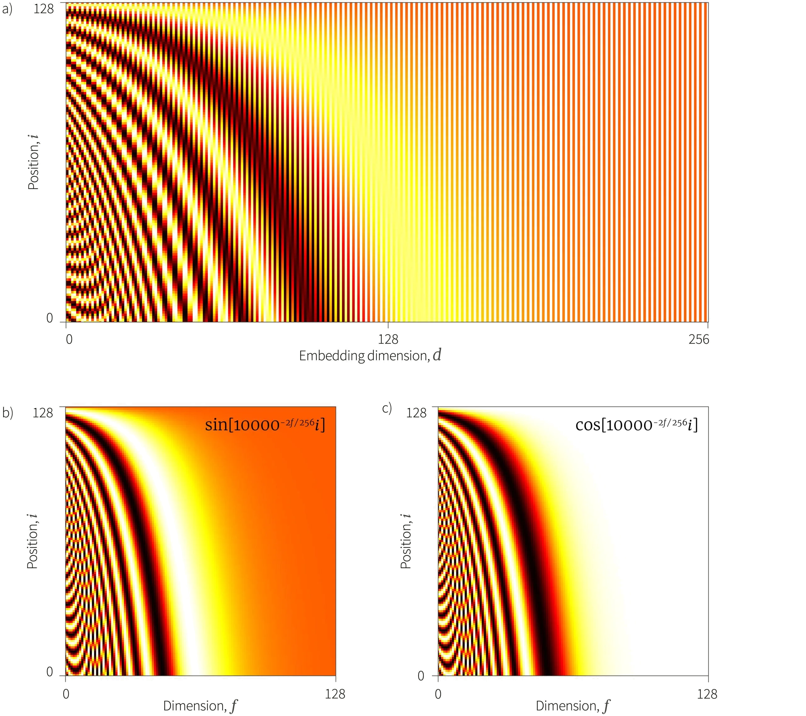
Figure 1. Sinusoidal position embeddings. a) The sinusoidal position embedding matrix $\boldsymbol\Pi$ is added to the data $\mathbf{X}$. There is a unique pattern associated at each position $i$ (rows of matrix). b) The even columns of the embedding matrix $\boldsymbol\Pi$ are made from terms of the form $\sin[\omega_{f} i]$ where the angular frequency $\omega_{f}$ decreases as a function of the dimension. c) The odd columns contain similar cosine terms.
One way to think about adding the matrix $\boldsymbol\Pi$ is that we are adding a different vector to the embedding $\mathbf{x}_{i}$ where this vector encodes the absolute position $i$. So if the same word occurs at different positions in the sequence, it would have two different embeddings. For this reason, this sinusoidal encoding is considered an absolute position embedding.
This scheme is worth examining closely. In the self-attention mechanism we apply linear transformations $\boldsymbol\Phi_{q}$ and $\boldsymbol\Phi_{k}$ to $\mathbf{X}+\boldsymbol\Pi$ and then compute dot products between every pair of columns in the resulting matrices. We’ll now consider several interesting properties that emerge we apply linear transformations to this sinusoidal embedding and take dot products.
Separating position and word embeddings: At first sight, adding the position embeddings to the data seems a bad idea; we probably need both the word embedding and the position embedding without having them hopelessly entangled. However, this is not necessarily a problem. Since the embedding dimension $D$ is usually greater than the maximum sequence length $I$ (e.g., BERT used D=1024, I=512), it is possible for the system to learn word embeddings that lie outside the subspace of the position embeddings. If this were the case, the system could recover the word embeddings by learning linear transformations $\boldsymbol\Phi_{q}$ and $\boldsymbol\Phi_{k}$ where the null-space spans the position embeddings. Similarly, the system could recover the position embeddings.
Down-weighting distant elements: The dot product between the position encodings $\boldsymbol\pi_{i}$ and $\boldsymbol\pi_{j}$ at different positions $i$ and $j$ (i.e. rows of $\boldsymbol\Pi)$ gets smaller as the relative position $|i-j|$ increase (figure 2). So if the system were to retrieve the position embeddings using a linear transform as described above, it could create an attention matrix that increasingly down-weights attention between elements as they become more distant when it computes the dot products.
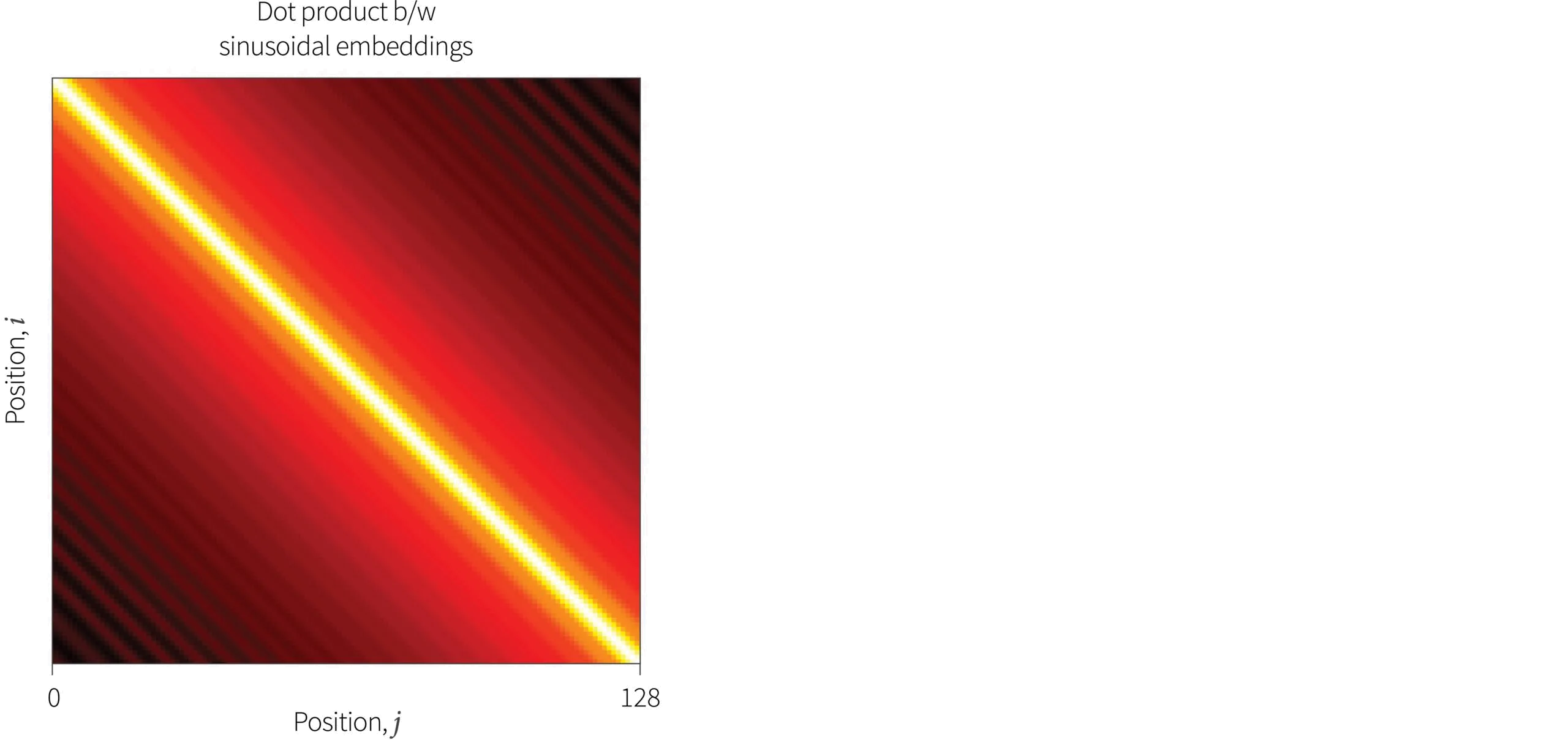
Figure 2. Dot products between sinusoidal embeddings from figure 1a. The magnitude generally decreases as function of the distance $|i-j|$. This is monotonic for the first 51 entries, but there is also a small oscillatory component that becomes more prominent at large distances.
Relative vs. absolute positions: We have added a unique embedding $\boldsymbol\pi_{i}$ at each absolute position $i$. However, it’s possible to transform the embedding $\boldsymbol\pi_{i}$ at position $i$ to that at relative position $i+j$ using a linear operation. To see this, consider the embeddings $\left(\sin[\omega_{f}i]\;\;\cos[\omega_{f} i]\right)^{T}$ at word position $i$ and two adjacent dimensions $d$ and $d+1$ of the embedding. Applying the following linear transform we get:
\begin{eqnarray}\begin{pmatrix}\cos[\omega_{f} j]&\sin[\omega_{f} j]\\-\sin[\omega_{f} j]&\cos[\omega_{f} j]\end{pmatrix}\begin{pmatrix}\sin[\omega_{f} i]\\\cos[\omega_{f} i]\end{pmatrix} &=&\begin{pmatrix}\cos[\omega_{f} j]\sin[\omega_{f} i]+ \sin[\omega_{f} j]\cos[\omega_{f} i]\\-\sin[\omega_{f} j]\sin[\omega_{f} i]+\cos[\omega_{f} j]\cos[\omega_{f} i]\end{pmatrix}\nonumber \\ &=&\begin{pmatrix}\sin[\omega_{f} (i+j)]\\\cos[\omega_{f} (i+j)]\end{pmatrix} \tag{4}\end{eqnarray}
where we have used the trigonometric addition identities. So by applying the appropriate linear transformation, the system can transform the position encoding at position $i$ to that at position $i+j$. If it did this for just the queries, then the dot products between position vectors would take a maximum value at a relative offset of $j$ rather than 0.
Note that all of the above is supposition; the trained network does not necessarily do any of these things. The point is that these capabilities are available to it if it chooses to use them.
Learned absolute position embeddings
We’ve seen that it’s possible to use sinusoidal embeddings for which the linear projections and dot-products have useful properties. An obvious next step is to learn the position embedding matrix $\boldsymbol\Pi$ during training. This approach was also tried in the original transformer paper and adopted by subsequent encoder models like BERT and GPT-2.
The advantage of learning the position embeddings is that we can potentially capture more complex properties. The disadvantage is that it adds a lot of extra parameters to the model, and once learned, the model cannot be extended to longer sequence lengths.
It’s interesting however, to test if the learned position embeddings capture the desirable properties of the sinusoidal embeddings. Wang and Chen (2020) compared the cosine similarities (closely related to dot products) between embeddings at different relative distances (figure 3). For GPT-2 the similarity of the embeddings decreases as a function of distance for small distances with a periodic component at larger distances. For BERT, the results are more noisy and complicated.
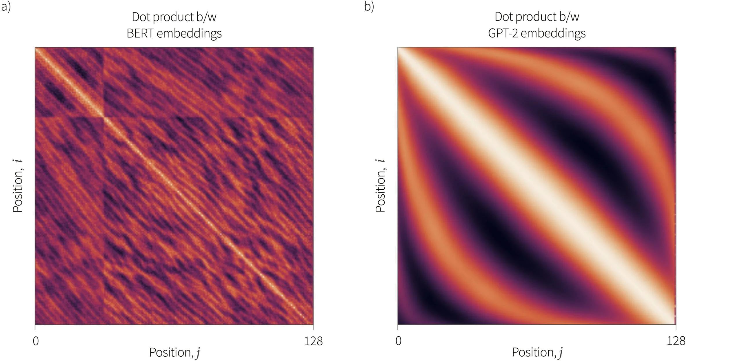
Figure 3. Dot products between learned embeddings from Bert and GPT2. a) BERT — the pattern is very noisy and there is a discontinuity due to the training process which has two phases in which the first phase uses only shorter sequences. Within the top-left region, there is a decreasing oscillatory pattern as a function of the difference $|i-j|$ in position b) GPT-2 — the dot products of the embedding show a smooth decreasing oscillatory pattern as a function of distance $|i-j|$. Adapted from Wang And Chen (2020)
They also examined if it is possible to predict the absolute positions by applying linear regression to the learned embedding. For the BERT embeddings, the error in these predictions is large, for the GPT-2 embeddings very small, and for the sinusoidal embeddings zero. The same experiment can be done by regressing pairs of position embeddings to predict relative position. Here, the error is again greatest for the BERT embeddings, but this time, the GPT-2 embeddings outperform the pre-defined sinusoidal embeddings.
Directly modifying the attention matrix
Adding position embeddings modifies the self-attention calculation to:
\begin{equation}\bf Sa [\mathbf{X}] = \bf Softmax\left[\frac{((\mathbf{X}+\boldsymbol\Pi)\boldsymbol\Phi_{q})((\mathbf{X}+\boldsymbol\Pi)\boldsymbol\Phi_{k})^{T}}{\sqrt{d_{q}}}\right](\mathbf{X}+\boldsymbol\Pi)\boldsymbol\Phi_{v}. \tag{5}\end{equation}
The position matrix modifies both the attention matrix (the softmax term) and the computation of the values. There have been a number of studies in which the latter modification is dropped so that just the attention matrix is changed:
\begin{equation}\bf Sa [\mathbf{X}] = \bf Softmax\left[\frac{((\mathbf{X}+\boldsymbol\Pi)\boldsymbol\Phi_{q})((\mathbf{X}+\boldsymbol\Pi)\boldsymbol\Phi_{k})^{T}}{\sqrt{d_{q}}}\right]\mathbf{X}\boldsymbol\Phi_{v}. \tag{6}\end{equation}
In these circumstances, the position information is usually added at every layer as it is only represented very implicitly in the output of the computation.
Let’s consider the un-normalized and pre-softmax attention matrix:
\begin{equation}\tilde{\mathbf{A}} = ((\mathbf{X}+\boldsymbol\Pi)\boldsymbol\Phi_{q})((\mathbf{X}+\boldsymbol\Pi)\boldsymbol\Phi_{k})^{T}, \tag{7}\end{equation}
which has elements:
\begin{eqnarray}\tilde{a}_{i,j} &=& ((\mathbf{x}_{i}+\boldsymbol\pi_{i})\boldsymbol\Phi_{q})((\mathbf{x}_{j}+\boldsymbol\pi_{j})\boldsymbol\Phi_{k})^{T}\nonumber \\&=& \underbrace{\mathbf{x}_{i}\boldsymbol\Phi_q\boldsymbol\Phi_{k}^{T}\mathbf{x}_{j}^{T}}_\text{content-content}+\underbrace{\mathbf{x}_{i}\boldsymbol\Phi_q\boldsymbol\Phi_{k}^{T}\boldsymbol\pi_{j}^{T}}_{\text{content-position}}+\underbrace{\boldsymbol\pi_{i}\boldsymbol\Phi_q\boldsymbol\Phi_{k}^{T}\mathbf{x}_{j}^{T}}_{\text{position-content}}+\underbrace{\boldsymbol\pi_{i}\boldsymbol\Phi_q\boldsymbol\Phi_{k}^{T}\boldsymbol\pi_{j^{T}}}_{\text{position-position}},\label{eq:attention_breakdown} \tag{8}\end{eqnarray}
where we can see that each element has four contributions in which the position embedding $\boldsymbol\pi$ and the content vector $\mathbf{x}$ interact differently. This expression has been modified in various ways
Untied embeddings: One simple modification is to decouple or untie the content and position components rather than add them together before projection. A simple way to do this is to remove the terms where they interact and to use a separate linear transform for each to give:
\begin{equation}\tilde{a}_{i,j} = \underbrace{\mathbf{x}_{i}\boldsymbol\Phi_q\boldsymbol\Phi_{k}^{T}\mathbf{x}_{j}^{T}}_\text{content-content}+\underbrace{\boldsymbol\pi_{i}\boldsymbol\Psi_q\boldsymbol\Psi_{k}^{T}\boldsymbol\pi_{j}^{T}}_{\text{position-position}}. \tag{9}\end{equation}
Relative embeddings: Another modification is to directly inject information about the relative position. For example, Shaw et al. (2018) add a term $\boldsymbol\pi_{|i-j|}$ which depends on the position difference.
\begin{equation}\label{eq:rel_pos_shaw}\tilde{a}_{i,j} = \underbrace{\mathbf{x}_{i}\boldsymbol\Phi_q\boldsymbol\Phi_{k}^{T}\mathbf{x}_{j}^{T}}_\text{content-content}+\underbrace{\mathbf{x}_{i}\boldsymbol\Phi_q\boldsymbol\pi_{i-j}^{T}}_{\text{content-position}}. \tag{10}\end{equation}
where a different position vector $\boldsymbol\pi_{i-j}$ is learned for each signed position offset $i-j$ where this offset is usually clipped so after a certain distance, all terms are the same. Note that this position vector is defined directly in the space of the keys rather than projected into it1.
Raffel et al. (2019) simplified this further by simply adding a learnable scalar $\pi_{|i-j|}$ to the attention matrix
\begin{equation}\tilde{a}_{i,j} = \underbrace{\left(\mathbf{x}_{i}\boldsymbol\Phi_q\boldsymbol\Phi_{k}^{T}\mathbf{x}_{j}^{T}\right)}_\text{content-content} + \pi_{i-j}. \tag{11}\end{equation}
where $\pi_{i-j}$ is a different scalar for each signed offset $i-j$. Relative position information has also been combined directly in other ways various other ways such as simply multiplying the attentions by a modifying factor $\pi_{|i-j|}$:
\begin{equation}\tilde{a}_{i,j} = \underbrace{\left(\mathbf{x}_{i}\boldsymbol\Phi_q\boldsymbol\Phi_{k}^{T}\mathbf{x}_{j}^{T}\right)}_\text{content-content}\cdot \pi_{|i-j|}. \tag{12}\end{equation}
where $\pi_{i-j}$ is a different scalar for each absolute offset $|i-j|$.
Finally, we note that pre-defined sinusoidal embeddings have also been used in a system based on equation 10 (where $\boldsymbol\pi_{ij}$ now contains sinusoidal terms in relative position $i-j$) and also in more complex ways.
Combining ideas: Many schemes combine have proposed position embeddings that combine the ideas of (i) only retaining certain terms from equation 8, (ii) using different projection matrices for the content and position embeddings, and (iii) using relative embeddings. For example, in DeBERTa they use:
\begin{equation}\tilde{a}_{i,j} =\underbrace{\mathbf{x}_{i}\boldsymbol\Phi_q\boldsymbol\Phi_{k}^{T}\mathbf{x}_{j}^{T}}_\text{content-content}+\underbrace{\mathbf{x}_{i}\boldsymbol\Phi_q\boldsymbol\Psi_{k}^{T}\boldsymbol\pi_{i-j}^{T}}_{\text{content-position}}+\underbrace{\boldsymbol\pi_{j-i}\boldsymbol\Psi_q\boldsymbol\Phi_{k}^{T}\mathbf{x}_{j}^{T}}_{\text{position-content}}. \tag{13}\end{equation}
where they drop the position-position term and have a different relative embedding $\boldsymbol\pi_{i-j}$ for each signed offset $i-j$ between the positions.
Summary
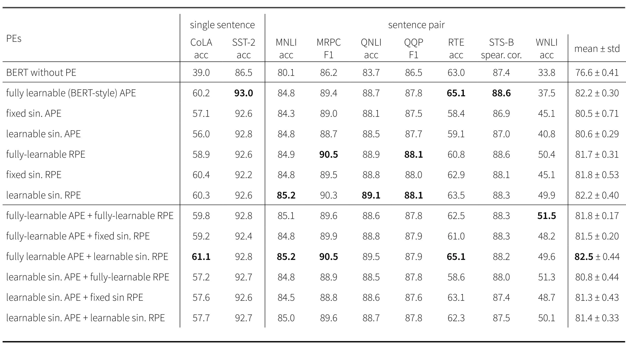
Figure 4. Empirical performance of different downstream tasks using BERT with different position embeddings. Absolute position embeddings (APE) are compared to relative position embeddings (RPE). Learned embeddnings are compared to sinusoidal embeddings, and a variant of sinusoidal embeddings in which the base of the angular frequency $10000$ is replaced with a learned value (see equation 2). Reproduced from Wang et al., 2021
In this section we have provided a brief overview of how position information is added into transformers. At the time of writing, it is not clear which of these position embedding schemes is empirically superior. For downstream tasks on BERT, relative position embeddings generally perform better than absolute position embeddings, but there does not seem to be much difference between sinusoidal embeddings and learned embeddings. To learn more about position embeddings, consult this survey paper.
Extending transformers to larger sets of inputs
In the second part of this blog, we consider modifications to the self-attention mechanism that make it more efficient as the sequence length increases. The self-attention mechanism takes $I$ inputs $\mathbf{x}_{i}$ and returns $I$ modified outputs. In this process, each input $\mathbf{x}_{i}$ interacts with one another; each output is a weighted sum of the values corresponding to every input, where the weights depend on how much the input attends to every other input. As such, the transformer naturally has quadratic complexity in the size $I$ of the input sequence.
However, there are some situations in which we might expect this input set to be extremely large. In NLP, we may wish to summarize long documents or answer questions about a body of documents. In other modalities like vision or audio processing, the data can also be of extremely high dimension. In these circumstances, the quadratic complexity of the attention mechanism can become the limiting factor and a sub-field has emerged that tries to address this bottleneck.
In this section, we review three lines of work. First, we discuss methods that aim to reduce the size of the attention matrix. Second, we review approaches that introduce sparsity into the attention matrix. Finally, we present methods that treat the self-attention computation as a kernel function and try to approximate this to create algorithms with linear complexity in the sequence length.
Reducing size of attention matrix
One simple idea to make self-attention more efficient is to reduce the size of the attention matrix. In memory compressed attention, a strided convolution is applied to the keys and values so the self-attention operation becomes:
\begin{equation} \bf Sa[\mathbf{X}] = \bf Softmax\left[\mathbf{X}\boldsymbol\Phi_{q}(\boldsymbol\theta_{k}\circledast\mathbf{X}\boldsymbol\Phi_{k})^{T} \right](\boldsymbol\theta_{v}\circledast\mathbf{X}\boldsymbol\Phi_{v}), \tag{14}\end{equation}
where $\boldsymbol\theta_{k}$ and $\boldsymbol\theta_{v}$ are the convolution kernels. If the stride $s$ is the same as the kernel size, then the effect is to take a learned weighted average of nearby key/value vectors and the resulting attention matrix reduces to size $I\times I/s$ (figure 5).
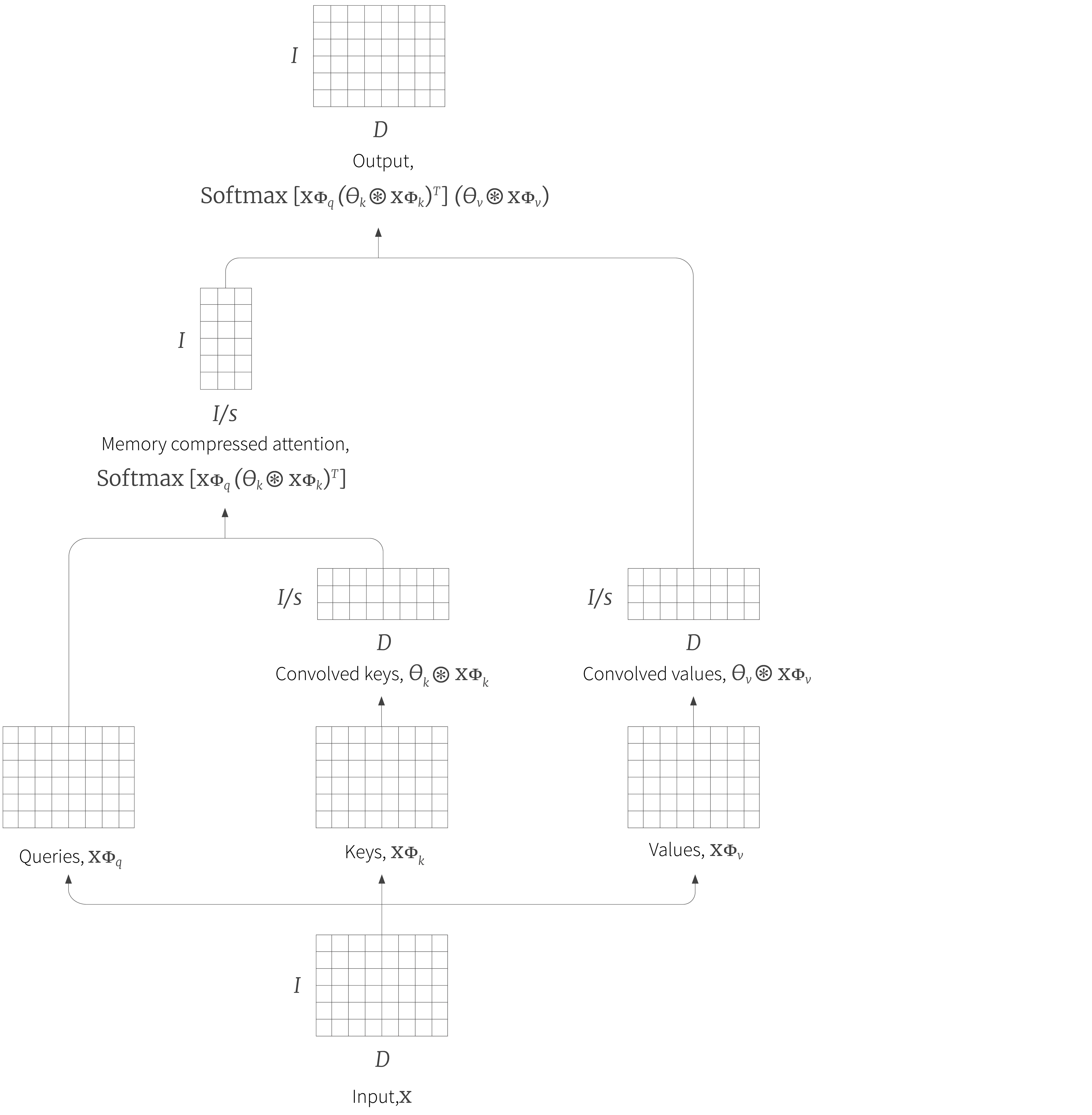
Figure 5. Memory compressed attention. One approach to reducing the size of the attention matrix is to apply strided convolution to the keys and values. If the is stride $s$ then the attention matrix becomes size $I\times I/s$. In practice, the kernel size is the same as the stride, so each input attends to weighted sums of neighboring inputs, rather than the inputs themselves.
The Linformer applies a very similar trick that is motivated by the observation that the self-attention mechanism is often low-rank in practice. Consequently, we can reduce the complexity of the calculation by projecting the keys and value into a learned subspace:
\begin{equation} \bf Sa[\mathbf{X}] = \bf Softmax\left[\mathbf{X}\boldsymbol\Phi_{q}(\boldsymbol\Psi_{k}\mathbf{X}\boldsymbol\Phi_{k})^{T} \right](\boldsymbol\Psi_{v}\mathbf{X}\boldsymbol\Phi_{v}), \tag{15}\end{equation}
where $\boldsymbol\Psi_{k}$ and $\boldsymbol\Psi_{v}$ are the $I/s\times I$ projection matrices for the keys and values respectively.
Making the attention matrix sparse
Another approach to making attention more computationally efficient is to constrain the attention computation so that every input does not attend to every other input. In local attention the inputs are divided into disjoint groups of neighbours and each block is passed through a separate self-attention mechanism before recombining (figure 6) In this way, inputs within the same block only attend to one another. Of course, this has the disadvantage that elements that are far from each other in the sequence never interact with one another, but alternating transformer layers that use local and full attention solves this problem.
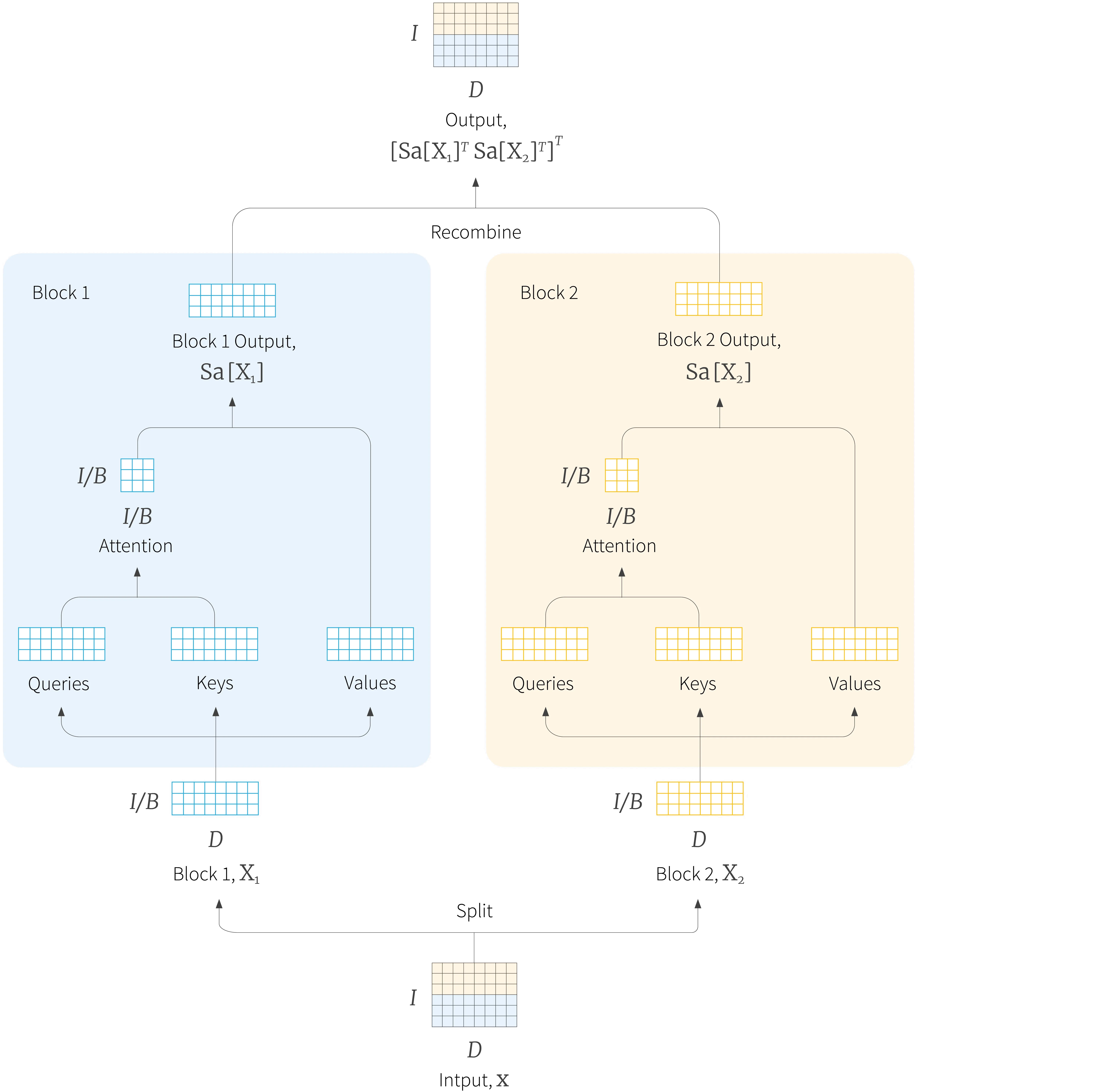
Figure 6. Local attention. Adjacent groups of inputs (blue and yellow rows) are processed by separate self-attention mechanisms and then re-combined.
Local attention can be visualized by plotting a matrix showing interaction of the queries and keys (figure 6). Note that for the decoder version, we also employ masked self-attention so each query can only attend to keys that have the same index or less and there are no interactions in the upper triangular portion.

Figure 7. Local self-attention can be visualized in terms of which queries interact with each keys, which we refer to as an interaction matrix. a) In the encoder version, the dot product is calculated between every query and key in a local block. b) In the decoder version, the block structure is retained, but dot products are not computed between queries and keys that are further along in the sequence.
Visualizing attention in this way leads naturally to the idea of using a convolutional structure (figure 7), in which each input only interacts with the nearest few inputs (or nearest preceding inputs for decoders). When used alone, this will mean that it may take many layers for information to propagate along the sequence. Again, this drawback can be remedied by alternating layers with the convolutional attention patterns and layers with full attention. Indeed, this is what is done in GPT-3. A different approach that maintains the overall sparsity is to use dilated convolutions with different dilation rates in different layers (figure 7b-c), or by introducing layers where some a few of the queries interact with every key (figure 7d). Collectively, these methods are referred to as sparse transformers.

Figure 8. Sparse transformers. a) Queries only interact with neighbouring keys, which gives the interaction matrix a convolutional structure. This is the decoder version, so all elements in the top-right triangular portion of the matrix are empty. b-c) To allow distant inputs to interact with each other more efficiently, transformers using the basic convolutional structure can be alternated with dilated convolutions with different dilatation rates. d) Alternatively, some layers may allow a subset of inputs to interact with all of the previous inputs.
The Longformer also used a convolutional structure which is sometimes dilated, but simultaneously allowed some keys to and queries to interact with all of the others (figure 9a). This was referred to as global attention and the positions correspond to special tokens such as the $<$cls$>$ token in BERT or special tokens in question answering tasks that delimit the question and answer. Note that global attention can only be used in encoder models since elements attend to every other element and hence see ahead in the sequence.
A natural extension of this method is to define some new content embeddings which attend to all of the keys and queries, but do not themselves correspond to any individual tokens in the input (figure 9). This is known as the extended transformer construction (ETC). These additional global content embeddings act as a kind of memory, which can both receive and broadcast information from all of the elements and are combined with a sparse convolutional pattern which ensures strong interactions between nearby inputs. The BigBird model took this idea by one step further by also adding sparse random connections between elements to help ensure the rapid mixing of information from different parts of the sequence.
One notable complication of using global content embeddings occurs if it is combined with relative attention; there is no relative offset between the global and regular elements, and so special relative position embeddings are learned for mapping to, from, and between, the global content embeddings.

Figure 9. Combining global and local attention. a) In the Longformer, a convolutional structure is used, but some inputs attend to every other input. These are chosen to correspond to special input tokens such as the $<$cls$>$ token in BERT. b) In the extended transformer construction extra global content embeddings are added which do not correspond to any of the input tokens, but act as global memory through which tokens far apart in the sequence can interact. c) In BigBird, random connections between the inputs are also added to this structure.
In this section we have reviewed approaches that make self-attention more efficient, by limiting the interaction between different inputs. Note that all of these methods use pre-defined sparsity patterns. There is also another line of research that attempts to learn the sparsity pattern. This includes the routing transformer, reformer and Sinkhorn transformer.
Kernelizing attention computation
A third approach to making self-attention more efficient it to approximate the attention computation using Kernel methods. The premise is that the dot product attention for the $i^{th}$ query can thought of as a special case of the following computation:
\begin{equation}\mathbf{x}_{i}^{\prime} = \frac{\sum_{j=1}^{I}\mbox{sim}[\mathbf{x}_{i}\boldsymbol\Phi_{q}, \mathbf{x}_{j}\boldsymbol\Phi_{k}]\mathbf{x}_{j}\boldsymbol\Phi_{v}}{\sum_{j=1}^{I}\mbox{sim}[\mathbf{x}_{i}\boldsymbol\Phi_{q}, \mathbf{x}_{j}\boldsymbol\Phi_{k}]} \tag{16}\end{equation}
where $\mbox{sim}[\bullet,\bullet]$ returns a measure of similarity between the two arguments. For dot-product self-attention, this is defined as $\mbox{sim}[\mathbf{x}_{i}\boldsymbol\Phi_{q}, \mathbf{x}_{j}\boldsymbol\Phi_{k}] = \exp[\mathbf{x}_{i}\boldsymbol\Phi_{q}(\mathbf{x}_{j}\boldsymbol\Phi_{k})^{T}]$.
We now treat this similarity as a kernel function, and as such it can be expressed as the dot product of non-linear transformations $\bf z[\bullet]$ of the inputs
\begin{equation} \mbox{sim}[\mathbf{x}_{i}\boldsymbol\Phi_{q}, \mathbf{x}_{j}\boldsymbol\Phi_{k}] = \bf z[\mathbf{x}_{i}\boldsymbol\Phi_{q}]\bf z[\mathbf{x}_{j}\boldsymbol\Phi_{k}]^{T}, \tag{17}\end{equation}
which means that the output becomes:
\begin{eqnarray}\mathbf{x}_{i}^{\prime} &=& \frac{\sum_{j=1}^{I}\bf z [\mathbf{x}_{i}\boldsymbol\Phi_{q}]\bf z [\mathbf{x}_{j}\boldsymbol\Phi_{k}]^{T}\mathbf{x}_{j}\boldsymbol\Phi_{v}}{\sum_{j=1}^{I}\bf z[\mathbf{x}_{i}\boldsymbol\Phi_{q}]\bf z[\mathbf{x}_{j}\boldsymbol\Phi_{k}]^{T}}\nonumber \\&=&\frac{\bf z[\mathbf{x}_{i}\boldsymbol\Phi_{q}]\sum_{j=1}^{I}\bf z[\mathbf{x}_{j}\boldsymbol\Phi_{k}]^{T}\mathbf{x}_{j}\boldsymbol\Phi_{v}}{\bf z[\mathbf{x}\boldsymbol\Phi_{q}]\sum_{j=1}^{I}\bf z[\mathbf{x}_{j}\boldsymbol\Phi_{k}]^{T}}, \tag{18}\end{eqnarray}
where we have used the associativity property of matrix multiplication between the first and second lines.
If we could find $\bf z[\bullet]$ such that $\bf z[\mathbf{x}_{i}\boldsymbol\Phi_{q}]\bf z[\mathbf{x}_{j}\boldsymbol\Phi_{k}]^{T} = \exp[\mathbf{x}_{i}\boldsymbol\Phi_{q}(\mathbf{x}_{j}\boldsymbol\Phi_{k})^{T}]$, then this is much more efficient. We compute the terms in the sums once and then compute each $\mathbf{x}_{i}$ term separately with a matrix multiplication. It turns out that such a non-linear transform $\bf z[\bullet]$ does indeed exist, but unfortunately, it maps the argument to an infinite dimensional space. From a computational viewpoint, this is not very helpful!
We’ll describe two approaches that sidestep this problem. First, the linear transformer implicitly uses a different measure of similarity $\bf sim[\mathbf{a},\mathbf{b}] = \bf z[\mathbf{a}]\bf z[\mathbf{b}]^{T}$ by defining a function $\bf z[\bullet]$ which is more tractable. In particular, they use $\bf z[\mathbf{a}] = \bf elu[\mathbf{a}]+1$ where $\bf elu[\bullet]$ is the exponential linear unit which is a pointwise non-linearity. Second, the performer attempts to approximate the standard dot-product similarity using a finite dimensional mapping $\bf z[\bullet]$. The latter approach is empirically more successful, but this may be because the tricks for training transformers (see part III of this blog) do not transfer effectively to using a different similarity measure.
These approaches can be also adapted to decoders. Here, when we calculate the output corresponding to input $\mathbf{x}_{i}$ we only use the partial sums up to index $i$:
\begin{eqnarray}\mathbf{x}_{i}^{\prime} &=& \frac{\bf z[\mathbf{x}_{i}\boldsymbol\Phi_{q}]\sum_{j=1}^{i}\bf z[\mathbf{x}_{j}\boldsymbol\Phi_{k}]^{T}\mathbf{x}_{j}\boldsymbol\Phi_{v}}{\bf z[\mathbf{x}_{i}\boldsymbol\Phi_{q}]\sum_{j=1}^{i}\bf z[\mathbf{x}_{j}\boldsymbol\Phi_{k}]^{T}} \nonumber \\&=& \frac{\bf z[\mathbf{x}_{i}\boldsymbol\Phi_{q}]\mathbf{A}_{i}}{\bf z[\mathbf{x}_{i}\boldsymbol\Phi_{q}]\mathbf{b}_i}, \tag{19}\end{eqnarray}
where $\mathbf{A}_{i}$ and $\mathbf{b}_{i}$ represent the partial sums in the numerator and denominator respectively. If we initialize $\mathbf{A}_{0}$ and $\mathbf{b}_{0}$ to zero, then the we can compute all the terms efficiently by iterating:
\begin{eqnarray}\label{eq:transformer_rnn}\mathbf{A}_{i}&\leftarrow&\mathbf{A}_{i-1}+ \bf z[\mathbf{x}_{j}\boldsymbol\Phi_{k}]^{T}\mathbf{x}_{i}\boldsymbol\Phi_{v}\nonumber \\\mathbf{b}_{i}&\leftarrow&\mathbf{b}_{i-1}+ \bf z[\mathbf{x}_{j}\boldsymbol\Phi_{k}]^{T}\nonumber \\\mathbf{x}_{i}^{\prime}&\leftarrow& \frac{\bf z[\mathbf{x}_{i}\boldsymbol\Phi_{q}]\mathbf{A}_{i}}{\bf z[\mathbf{x}_{i}\boldsymbol\Phi_{q}]\mathbf{b}_i}. \tag{20}\end{eqnarray}
In conclusion, if we consider the interaction between the queries and keys to be a kernel function, we can replace this by the dot product of non-linear functions of the key and query. This leads naturally to a very efficient implementation for both encoder and decoder architectures.
Summary
In this section, we have reviewed three families of modifications that allow the self-attention mechanism to be extended to longer sequences without a quadratic increases in computation. To learn more about this area, consult this review paper.
Relation of dot-product self-attention to other models
In the previous sections, we have addressed the questions of how to encode position, and how to extend the transformer to longer sequence lengths. In this section, we shift gears and consider the relationship between the self-attention mechanism and other models. We’ll also consider alternatives to the self-attention mechanism.
Self-attention as an RNN
The first connection that we will draw is between the self-attention decoder and recurrent neural networks (RNNs). In the final part of the previous section, we re-interpreted the dot-product self-attention mechanism as a kernel function $\mbox{k}[\bullet, \bullet]$:
\begin{equation}\mathbf{x}_{i}^{\prime} = \frac{\sum_{j=1}^{i}\mbox{k}[\mathbf{x}_{i}\boldsymbol\Phi_{q}, \mathbf{x}_{j}\boldsymbol\Phi_{k}]\mathbf{x}_{j}\boldsymbol\Phi_{v}}{\sum_{j=1}^{i}\mbox{k}[\mathbf{x}_{i}\boldsymbol\Phi_{q}, \mathbf{x}_{j}\boldsymbol\Phi_{k}]} = \frac{\sum_{j=1}^{i} \bf z[\boldsymbol\Phi_{q}\mathbf{x}_{i}]\bf z[\mathbf{x}_{j}\boldsymbol\Phi_{k}]^{T}\mathbf{x}_{j}\boldsymbol\Phi_{v}}{\sum_{j=1}^{i} \bf z[\mathbf{x}_{i}\boldsymbol\Phi_{q}]\bf z[\mathbf{x}_{j}\boldsymbol\Phi_{k}]^{T}}. \tag{21}\end{equation}
This means that the kernel function can be replaced by the dot product of non-linear functions $\bf z[\bullet]$ of the queries and keys and this led to the iterative computation in equation 20.
Viewed in this light, the decoder has an obvious mapping to an RNN. Each state is processed sequentially and the quantities $\mathbf{A}_{i}$ and $\mathbf{b}_{i}$ from equation 20 form the hidden state (figure 10). However, it turns out that to exactly replicate dot-product self-attention requires the function $\bf z[\bullet]$ to map its arguments to an infinite dimensional space. Hence, it is perhaps unsurprising that the transformer architecture out-performs the RNN in practice.

Figure 10. Transformer decoder as an RNN. If we treat the computation of the attention matrix as a kernel function, we can then re-express it in terms of the dot product $\bf z[\mathbf{x}{i}\boldsymbol\Phi{q}]\bf z[\mathbf{x}{j}\boldsymbol\Phi{k}]^{T}$ of non-linear functions $\bf z[\bullet]$ of the queries and keys. For a transformer decoder, this leads to an iterative computation where the tokens are processed sequentially. This can be interpreted as an RNN, where the state is embodied in the matrix $\mathbf{A}{i}$ and the vector $\mathbf{b}{i}$ containing the summation terms from equation 10.
Attention as a hypernetwork
A hypernetwork is a network that is used to predict the parameters of a second network that then performs the main task in hand. In part I of this tutorial, we already saw that the attention matrix can be interpreted as forming the weights of a network that maps the values to the outputs (figure 11). These weights are (i) non-negative, (ii) sparse (there is no interaction between the different dimensions of the values) and (iii) shared (the same weight is used for every dimension of the interaction between the $i^{th}$ value and the $j^{th}$ output). As such they form a hypernetwork with a particular structure.

Figure 11. Self attention computation for $I=3$ inputs $\mathbf{x}{i}$, each of which has dimension $D=4$. a) The input vectors $\mathbf{x}{i}$ are all operated on independently by the same weights $\boldsymbol\Phi_{v}$ (same color equals same weight) to form the values $\mathbf{x}{i}\boldsymbol\Phi{v}$. Each output is a linear combination of these values, where there is a single shared attention weight $a[\mathbf{x}{i}, \mathbf{x}{j}]$ that relates the contribution of the $i^{th}$ value to the $j^{th}$ output. b) Matrix showing block sparsity of linear transformation $\boldsymbol\Phi_{v}$ between inputs and values. c) Matrix showing sparsity of attention weights in the linear transformation relating values and outputs.
Viewed from this perspective, we might consider other mechanisms than dot-product self attention to create these weights (figure 12). The synthesizer uses a multi-layer perceptron $\bf MLP[\bullet]$ to create each row of the $I\times I$ matrix from input $\mathbf{x}_{i}$. This row is then passed through the softmax function to create the attention weights:
\begin{eqnarray} \mbox{Synthesizer}\left[\mathbf{X} \right] &=&\bf Softmax\left[\bf MLP[\mathbf{X}]\right] \mathbf{X}\boldsymbol\Phi_{v}\nonumber \\ &=&\bf Softmax\left[\bf Relu[\mathbf{X}\boldsymbol\Phi_{1}]\boldsymbol\Phi_{2}]\right] \mathbf{X}\boldsymbol\Phi_{v}\nonumber\end{eqnarray}
This is interesting since the rows of the attention matrix are no longer computed based on similarities between pairs of tokens, but just from each individual token alone. Surprisingly, it seems to work comparably well to the original dot-product self-attention mechanism.
A similar idea can be used to generate an attention matrix with convolutional structure. This belongs to the family of dynamic convolutions in which the convolution weights are themselves determined by the data. Part of the network block in the paper Pay less attention uses this approach. One advantage of this scheme is that there is no need for a position encoding; the convolution weights are determined by all of the inputs, and if we permute them, the result will be different.
Finally, it should be noted that linear transformers are also closely related to fast weight memory systems which are intellectual forerunners of hypernetworks.
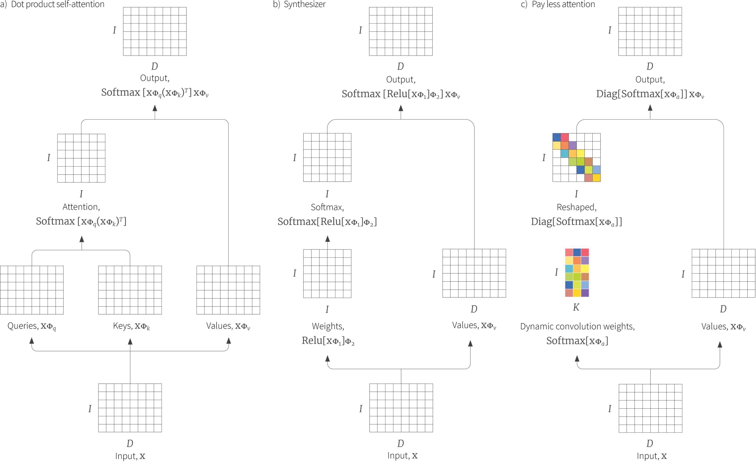
Figure 12. Attention as a hypernetworks. a) Original dot-product self-attention architecture. The attention matrix can be interpreted as forming weights that map the values $\mathbf{x}{i}\boldsymbol\Phi{v}$ to the outputs (see figure 11). b) The synthesizer removes dot-product attention and simply generates these weights using a multi-layer perceptron to generate an $I\times I$ matrix which has a softmax operator applied independently to each row. c) In the paper “Pay less attention”, a similar idea is employed to generate an attention matrix with a convolutional structure.
Attention as routing
A different way to think about self-attention is as a routing network. The attention matrix distributes (routes) each of the $I$ computed value vectors to the $I$ outputs. From this viewpoint, there is a connection between self-attention and capsule networks. Roughly speaking, a capsule network is intended to capture hierarchical relations in images, so lower network levels might detect facial parts (noses, mouths), which are then combined (routed) in higher level capsules that represent a face. One major difference is that capsule networks use routing by agreement. In self-attention, the elements $\mathbf{x}_{i}$ compete with each other for how much they contribute to output $j$ (via the softmax operation). In capsule networks, the higher levels of the network compete with each other for inputs from the lower levels.
Once we consider self-attention as a routing network, we can ask the question of whether it is necessary to make this routing dynamic (i.e, dependent on the data). Another variant of the synthesizer removed the dependence of the attention matrix on the inputs entirely and either used pre-determined random values or learned values (figure 13a). This performed surprisingly well across a variety of tasks.
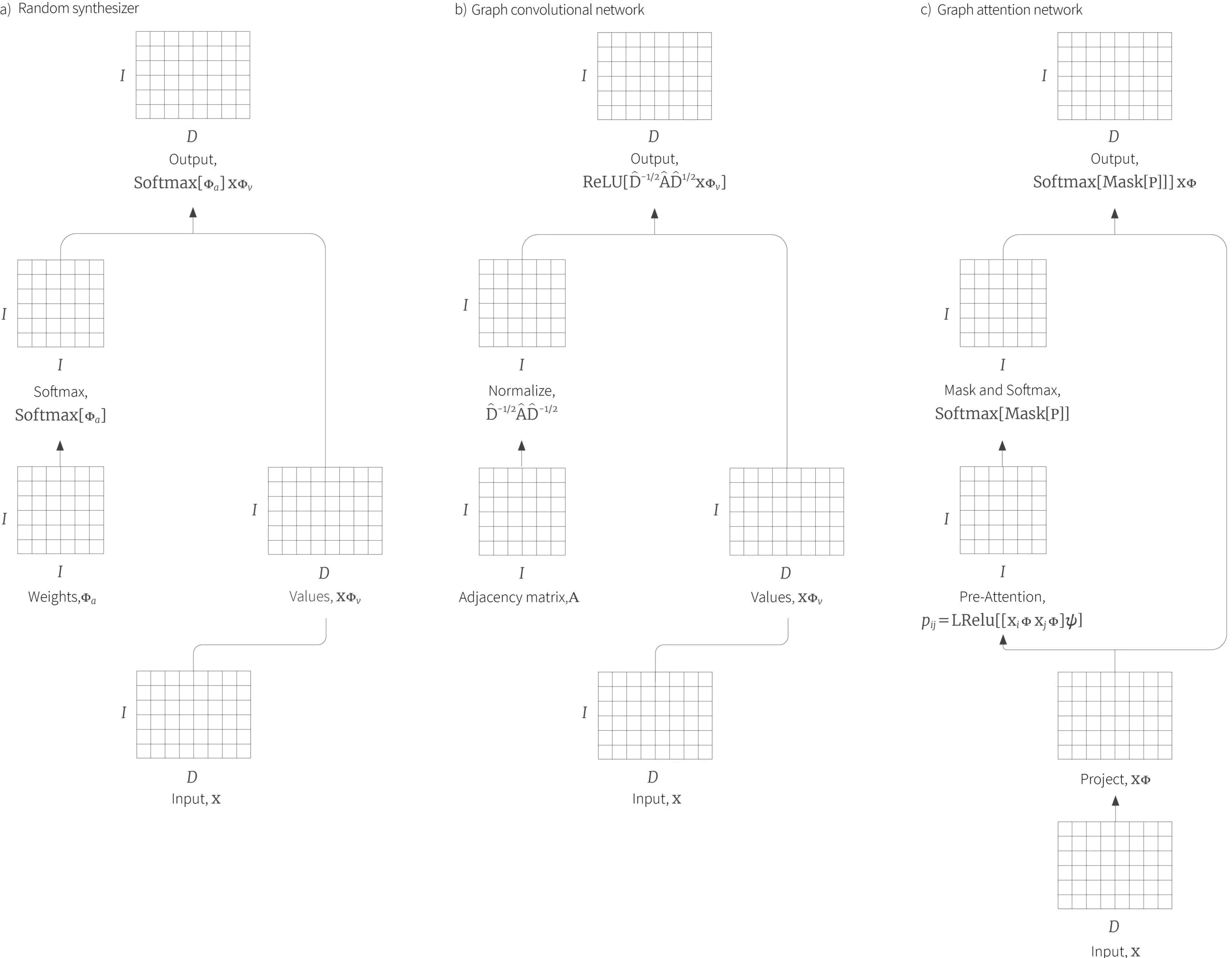
Figure 13. Attention as routing. a) The random synthesizer uses a pre-determined or learned attention matrix; it routes information between the inputs, but the routing does not depend on the inputs themselves b) In a graph convolutional network, the routing depends on the graph structure which is captured by the node adjacency matrix $\mathbf{A}$. This matrix $\hat{\mathbf{A}} = \mathbf{A}+\mathbf{I}$ and diagonal node degree matrix $\hat{\mathbf{D}}$ are both functions of this adjacency matrix. c) In a graph attention network, the connection between the inputs and the routing is restored (although it uses a different mechanism than dot-product self-attention). Here, the graph structure is also imposed via the function $\bf Mask[\bullet]$ which ensures that the contributions in the attention matrix are zero if there is no connection between the associated nodes.
Attention and graphs
Graph convolutional networks consider each input vector $\mathbf{x}_{i}$ to be associated with a node on a known graph, and process these nodes through a series of layers in which each node interacts with its neighbours. As such they have a close relationship to self-attention; they can be viewed as routing networks, but here the routing is determined by the adjacency matrix of the graph (figure 13b) and not the data.
Graph attention networks (figure 13c) combine both mechanisms; the routing depends both on the data (although using additive attention, not dot-product attention) and the graph structure (which is used to mask the attention matrix in a similar way to in masked self-attention in decoders).
Returning to the original self-attention mechanism, it is now clear that it can be viewed as a graph neural network on the complete graph, where the query tokens are the destination nodes and the key and value tokens are the source nodes.
Attention and convolution
Linear convolutions of the neighboring inputs in the sequence can be considered a special case of multi-head dot-product self attention with relative position embeddings. For example, consider using additive position embeddings so that the overall self-attention mechanism is given by:
\begin{equation}{\bf Sa}[\mathbf{X}] =\bf Softmax\left[(\mathbf{X}\boldsymbol\Phi_{q})(\mathbf{X}\boldsymbol\Phi_{k})^{T}+\boldsymbol\Pi\right]\mathbf{X}\boldsymbol\Phi_{v}, \tag{22}\end{equation}
where the matrix $\boldsymbol\Pi$ has a different learned value $\pi_{i-j}$ for each offset $|i-j|$. Now consider setting $\boldsymbol\Phi_{q}=\boldsymbol\Phi_k = \mathbf{0}$ and $\boldsymbol\Phi_{v}=\mathbf{I}$ to yield:
\begin{equation}{\bf Sa}[\mathbf{X}] =\bf Softmax\left[\boldsymbol\Pi\right]\mathbf{X}\nonumber. \end{equation}
If we now choose the relative position contributions $\pi_{i-j}$ to be very large for one offset $i-j$ and small for all of the others, the overall effect will be to create an attention matrix with zeros everywhere except within a single diagonal offset by $i-j$ from the center, where the values will be one. When applied to the data $\mathbf{X}$, this has the effect of shifting the rows of the value matrix by $j$. In a multi-head attention context, each head could learn a different offset. When the outputs of these heads are recombined using:
\begin{equation} {\bf MhSa}[\mathbf{X}] = \left[{\bf Sa}_{1}[\mathbf{X}]\;{\bf Sa}_{2}[\mathbf{X}]\;\ldots\;{\bf Sa}_{H}[\mathbf{X}] \right]\boldsymbol\Phi_{c}, \tag{23}\end{equation}
it is possible to choose $\boldsymbol\Phi_{c}$ so that all of the outputs from the $h^{th}$ self attention mechanism have the same weight and so we have effectively performed a convolution on the rows of $\mathbf{X}$.
To summarize, it is possible for a multi-head self attention with relative position embeddings to simulate convolution. This is particularly interesting when the transformer is applied to vision problems where convolutional networks are the standard. Indeed, there is some evidence that this is exactly what transformers are doing in vision tasks.
Attention vs. gating
A notable characteristic of the self attention mechanism and related models is that the processing divides into two paths, one of which is later used to modify the other. In attention, this modification takes the form of pre-multiplication by the attention matrix. However, there is another family of models which use one path to just modulate the magnitude of the other.
The gated linear unit (figure 14a) is an example of such a gating mechanism. The input $\mathbf{X}$ has a linear transformation $\boldsymbol\Phi_{u1}$ applied to it and the result is passed through a pointwise sigmoid function $\bf Sig[\bullet]$ . This maps the results to between zero and one so that they can be used to modulate the magnitude of the data $\mathbf{X}\boldsymbol\Phi_{u2}$ flowing down the other path, which have been subject to a a different linear transformation. The whole function is hence:
\begin{equation} \bf GLU[\mathbf{X}] = \bf Sig[\mathbf{X}\boldsymbol\Phi_{u1}]\odot \mathbf{X}\boldsymbol\Phi_{u2}. \tag{24}\end{equation}
Although the architecture is superficially similar, this is not really equivalent to a transformer, as each input $\mathbf{x}_{i}$ (row of $\mathbf{X}$) is treated independently. The gated MLP addresses this by modifying the architecture to incorporate a learned linear transformation $\boldsymbol\Psi$ that combines together the different inputs:
\begin{equation} \bf GMLP[\mathbf{X}] = (\bf Sig[\mathbf{X}\boldsymbol\Phi_{u1}]\odot \boldsymbol\Psi\mathbf{X}\boldsymbol\Phi_{u2})\boldsymbol\Phi_{v}. \tag{25}\end{equation}
as well as a final linear transform $\boldsymbol\Phi_{v}$ that remaps to the original dimensionality. This model again has the advantage that it does not need a position encoding; the inputs are mixed using $\boldsymbol\Psi$ and if we permute their order, the output will not just be a permutation of the input.
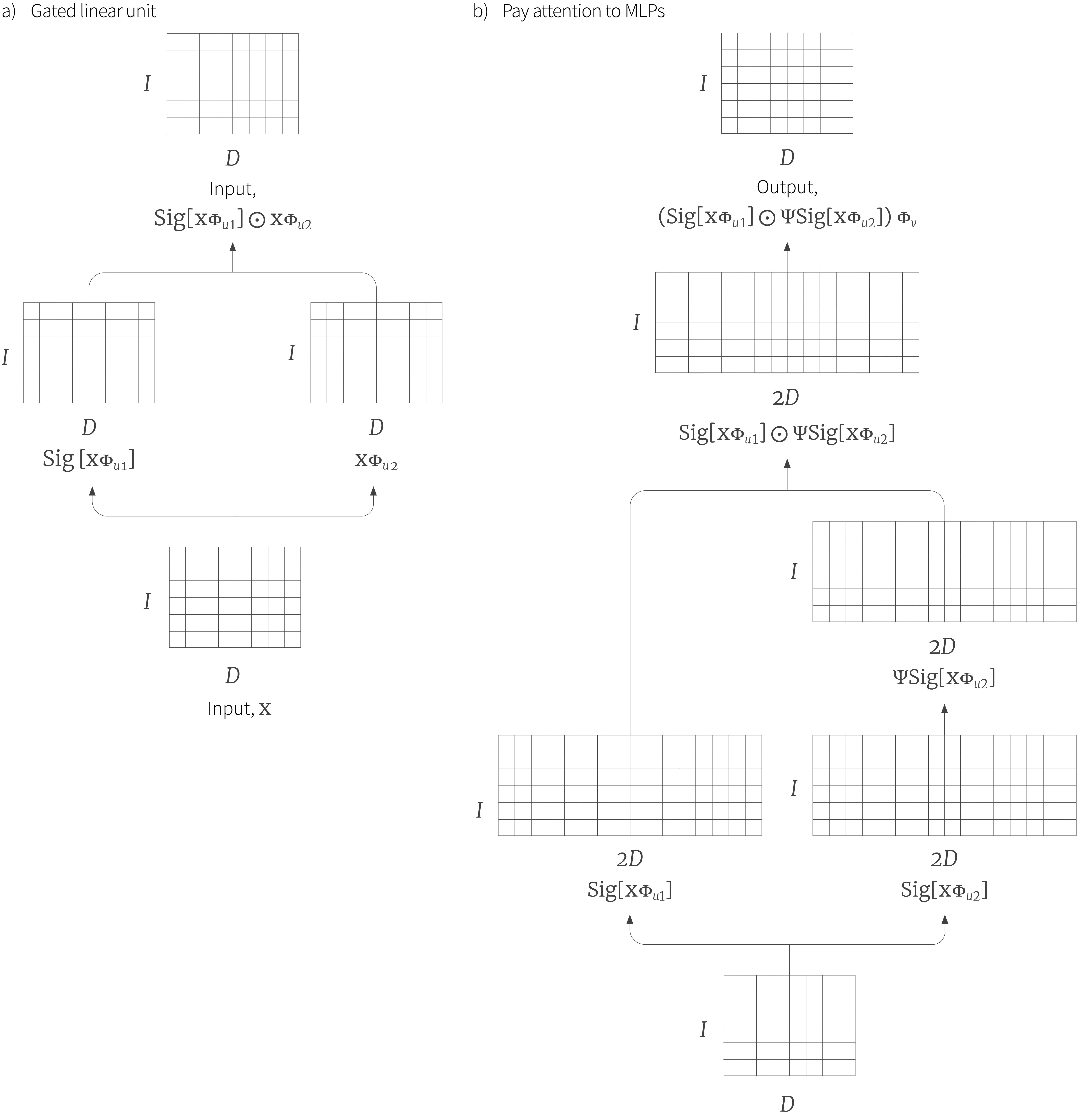
Figure 14. Gating networks. a) Gated linear unit. The dimensions of the inputs are combined using a linear transformations $\boldsymbol\Phi_{u1}$. The result is passed through pointwise sigmoid non-linearity that maps all the values to between 0 and 1. These are then pointwise multiplied with $\mathbf{X}\boldsymbol\Phi_{u2}$, so the left path acts to modulate the magnitude of elements in the right path. b) The gated MLP adapts this architecture so it is more equivalent to the transformer. Notably, the right hand path pre-multiplies the data by learned matrix $\boldsymbol\Psi$ which mixes the inputs.
Attention as memory retrieval
Finally, we’ll consider the relationship between Hopfield networks and the attention mechanism. A Hopfield network can retrieve a stored memory based on a query via an iteratve procedure in which the query is updated after interaction with the system. They were originally defined for binary vectors, but the modern Hopfield network extends the idea to continuous values.
Ramsauer et al. (2020) show that for a carefully defined Hopfield energy function, the update rule is equivalent to self-attention mechanism. The most natural way to think of this is in terms of encoder-decoder attention. The decoder queries memories from the encoder network. If viewed as a Hopfield network, the query-key attention computes a simple iteration of the memory retrieval. To complete the process, the output of the attention network should be feed back in as a new query until a stable state is reached (figure 15).
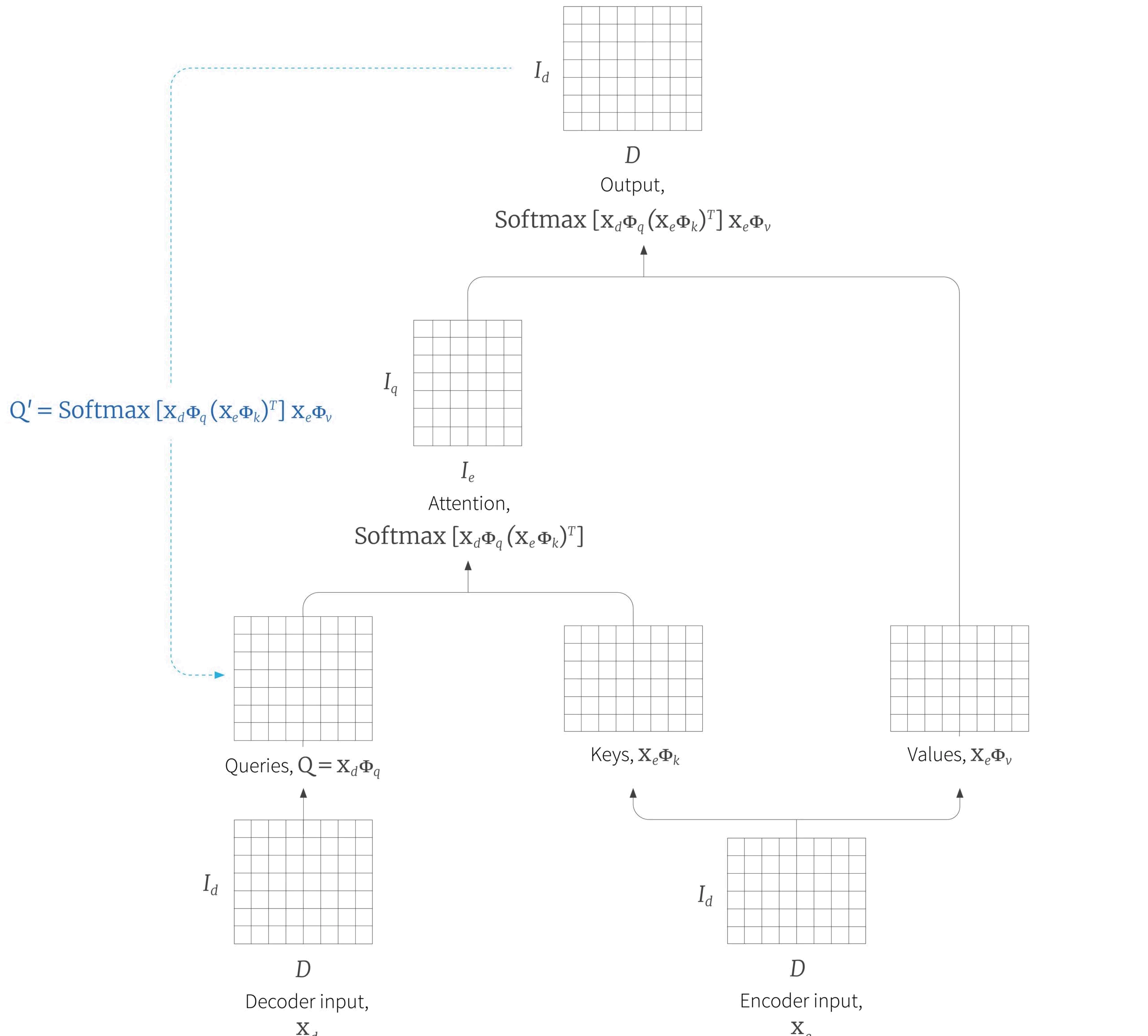
Figure 15. Attention as memory retrieval. The encoder-decoder attention module can be characterized of in terms of the decoder retrieving a memory from the encoder. One interpretation of this that it is a single step of the update rule of a modern Hopfield network. Viewed in this light, we might consider iterating the procedure by feeding the output of the attention mechanism back in as a new query repeatedly until the output stops changing.
Discussion
In this blog, we have discussed extensions to the basic self-attention mechanism. First, we discussed how to incorporate positional information, and then how to extend the self-attention mechanism to longer sequences. Finally, we have discussed the relationship between self-attention and a number of other models, including RNNs, CNNs, graph convolutional networks and Hopfield networks. We note that some caution is required here. Recent work has suggested that many of the variations of the original model do not necessarily yield consistent performance benefits.
In part III of this blog, we discuss how to train transformers in practice. To make training stable, a number of tricks are required including unusual learning rate scheduled, various forms of normalization, and careful initialization.
1 In fact they also modified the value terms in a similar way although their ablation study suggested that this did not contribute much
News
Meet Turing by RBC Borealis, an AI-powered text to SQL database interface
Tutorial #14: Transformers I: Introduction
Work with Us!
Impressed by the work of the team? RBC Borealis is looking to hire for various roles across different teams. Visit our career page now and discover opportunities to join similar impactful projects!
Careers at RBC Borealis