
In part I of this series of blogs we explored gradient flow (gradient descent with an infinitesimal step size) in linear models with least squares losses. We saw that it’s possible to derive expressions for the evolution of the parameters, loss, and predictions. Moreover, by examining these expressions it is possible to understand when the system is trainable and learn about the speed with which training converges.
In part II (this article) and part III, we apply these insights to neural networks. In this article, we show that, in the infinite width limit, a neural network behaves as if it is linear, and its training dynamics can be captured by the neural tangent kernel, or NTK for short. This can be computed in closed form for infinitely wide networks.
In part III, we use the neural tangent kernel to provide insights into the trainability and convergence of neural networks. We also treat the neural tangent kernel as a non-linear transformation of the input data, which allows us to reinterpret inference in neural networks as a kernel regression problem and make predictions in closed form without ever explicitly training the network.
Infinite width neural networks
We start by examining what happens when we increase the width of a neural network. For simplicity, we’ll assume that both the input $x$ and the output $y$ are scalar, and we’ll define the network as:
\begin{eqnarray}
\mathbf{h}_{1} &=& \mathbf{ReLU}\Bigl[\boldsymbol\beta_0 + \boldsymbol\omega_{0}x\Bigr]\nonumber\\
\mathbf{h}_{2} &=& \frac{1}{\sqrt{D}}\Bigl(\mathbf{ReLU}\Bigl[\boldsymbol\beta_1 + \boldsymbol\Omega_{1}\mathbf{h}_{1}\Bigr]\Bigr)\nonumber\\
y &=& \frac{1}{\sqrt{D}}\Bigl(\beta_2 + \boldsymbol\Omega_2 \mathbf{h}_{2}\Bigr),
\tag{1}
\end{eqnarray}
where $\mathbf{h}_{1},\mathbf{h}_{2}\in\mathbb{R}^{D}$ represents the activations of the $D$ hidden units in the first and second hidden layers, and $\mathbf{ReLU}[\bullet]$ represents the elementwise application of the standard ReLU function. The parameters consist of the biases $\boldsymbol\beta_0\in\mathbb{R}^{D}$, $\boldsymbol\beta_1\in\mathbb{R}^{D}$, $\beta_{2}\in\mathbb{R}$ and the weights $\boldsymbol\omega_{0}\in{R}^{D\times 1}$, $\boldsymbol\Omega_{1}\in{R}^{D\times D}$, and $\boldsymbol\Omega_{2}\in\mathbb{R}^{1\times D}$. This is a standard neural network with two hidden layers, except for the rescaling terms $1/\sqrt{D}$, which compensate for the increase in the width and prevents exploding activations/gradients when we initialize the weights from a standard normal distribution (i.e., they obviate the need for Xavier initialization). This is sometimes termed the NTK parameterization of a neural network.
Let’s consider training this data on $I=10$ data pairs $(x_{i},y_{i})$ where both inputs $x_i$ and targets $y_i$ are drawn from a standard normal distribution. We initialize the biases to zero and the weights from a standard normal distribution. We then apply stochastic gradient descent with momentum to train networks with different widths $D$. Figure 1 shows how the weights $\boldsymbol\Omega_{1}$ between the two hidden layers change during training for widths $D=10,50,1000$; as the width gets larger, individual parameters change less. This is expected since the responsibility for describing the finite dataset becomes distributed between more and more parameters, so the change in any given parameter is smaller.
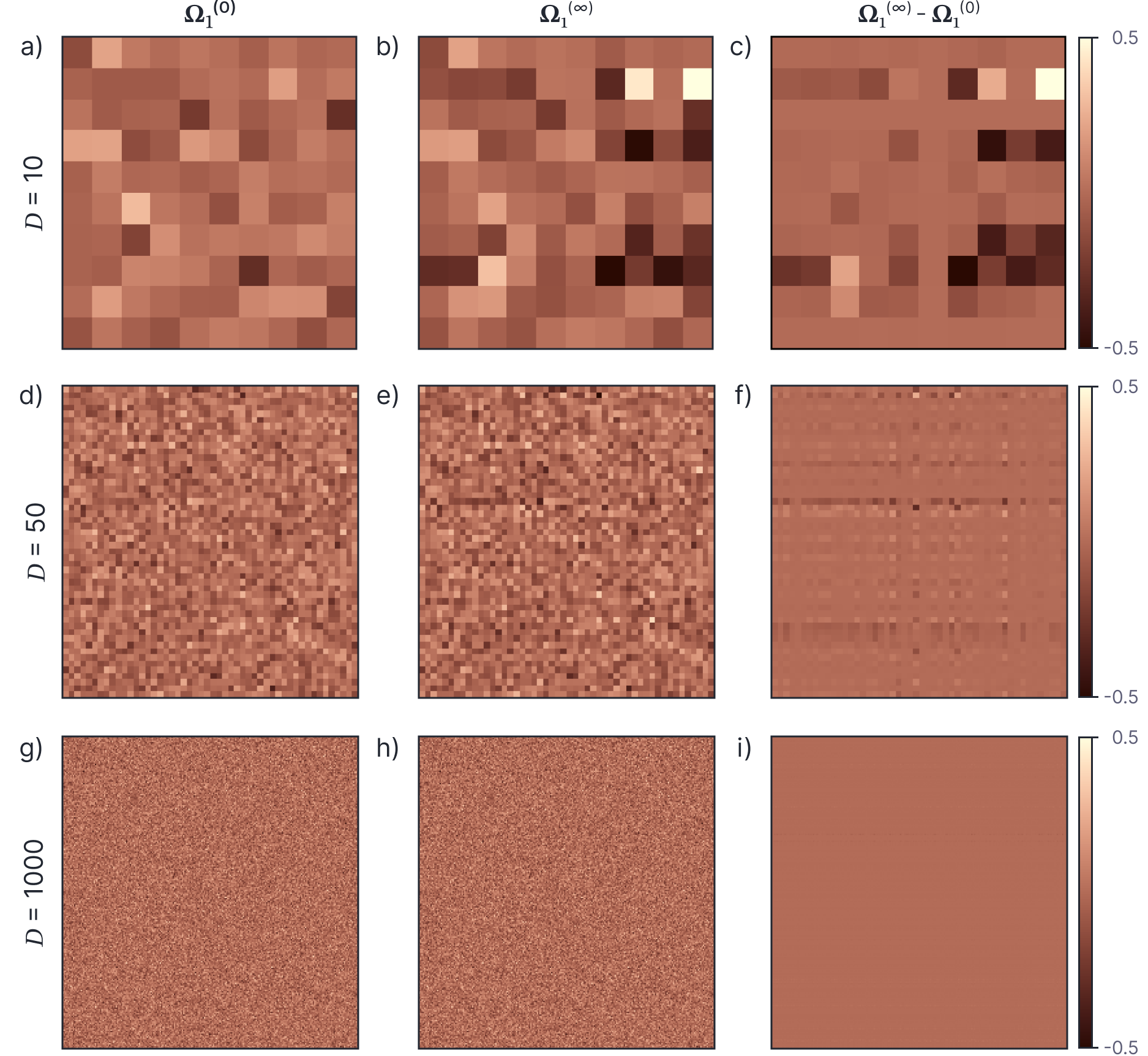
Figure 1. Change in weights in two layer neural network as the width $D$ changes. a) Weights $\boldsymbol\Omega_1$ between first and second hidden layers before training with width $D=10$. b) Weights $\boldsymbol\Omega_1$ after training. c) Change in weights during training. d-f) Weight matrix before training, weight matrix after training, and change in weight matrix for width $D=50$ and g-i) width $D=1000$. As the width increases, the individual weights change less, and at large widths are almost constant throughout training. Figure inspired by $\href{https://rajatvd.github.io/NTK/}{\color{blue} Dwaraknath(2019)}.$
One way to characterize the change is to look at the Frobenius norms of original weights and their changes. Figure 2a shows the norm of the initial weight matrices. This naturally increases as the width increases as the number of weights increases. Figure 2b depicts the norm of the change in weights. This is roughly constant; but this change is distributed across more parameters as the width increases, so the individual weights change less. We can characterize the tendency of the weights to remain nearly constant by the ratio of the norm of the change to the norm of the original weights (figure 2c). This decreases systematically as the width increases.

Figure 2. Change in weights in two layer neural network as the width $D$ changes. a) The Frobenius norm $|\boldsymbol\Omega^0_{1}|_{2}$ of the initial weight matrix increases as the width increases (there are more weights, each with the same amount of variation). b) The norm of the change in weights $|\boldsymbol\Omega^\infty_{1}-\boldsymbol\Omega^0_{1}|_{2}$ is roughly constant as the width increases (but this change is now distributed across more weights). c) Consequently, the norm of the change relative to the initial norm $|\boldsymbol\Omega^\infty_{1}-\boldsymbol\Omega^0_{1}|_{2}/|\boldsymbol\Omega^0_{1}|_{2}$ decreases with width.
Mathematical characterization of weight change
This diminishing change in individual weights as the network width increases can also been shown mathematically. For example, Du (2019) demonstrates this for a toy shallow network $\mbox{f}[x,\boldsymbol\phi]$ with $D$ hidden units that maps scalar input $x$ to scalar input $y$:
\begin{equation}
\mbox{f}[x,\boldsymbol\phi] = \frac{1}{\sqrt{D}}\sum_{d=1}^{D} \theta_{d} \cdot \mbox{a}\bigl[\phi_{d}x\bigr],
\tag{2}
\end{equation}
where $a[\bullet]$ is a Lipschitz activation function. We’ll assume that the weights $\theta_{d}$ that map from the hidden layer to the output are assigned randomly to $\pm 1$ and fixed, leaving $D$ parameters $\phi_d$ that map from the input to the hidden layer. These are initialized from a standard normal distribution. We’ll use a least squares loss function $L[\boldsymbol\phi]$ defined over $I$ training pairs $\{x_{i},y_{i}\}$.
\begin{equation}
L[\boldsymbol\phi] = \frac{1}{2}\sum_{i=1}^I\Bigl(\mbox{f}\bigl[x_{i},\boldsymbol\phi\bigl]-y_i\Bigr)^2.
\tag{3}
\end{equation}
With gradient flow, the evolution of a parameters $\boldsymbol\phi_{d}$ is defined by:
\begin{eqnarray}
\frac{d \phi_{d}}{dt} = – \frac{\partial L}{\partial \phi_d} = -\frac{1}{\sqrt{D}}\sum_{i=1}^I \Bigl(\mbox{f}\bigl[x_{i},\boldsymbol\phi\bigl]-y_i\Bigr)\theta_{d} x_i\cdot \mbox{a}^{\prime}\left[\phi_d x\right].
\tag{4}
\end{eqnarray}
Now consider the total change in a parameter $\phi_{d}$ over time:
\begin{equation}
\Bigl\lVert \phi_{d}[T]-\boldsymbol\phi_{d}[0] \Bigr\rVert_{2}\leq \int_{0}^{T} \left\lVert \frac{d \phi_{d}[t]}{dt} \right\rVert_2 dt = \mathcal{O}\left[\frac{1}{\sqrt{D}}\right],
\tag{5}
\end{equation}
because considering each term in the derivative in turn (i) $|\mbox{f}\bigl[\mathbf{x}_{i},\boldsymbol\phi\bigl]-y_i|$ decreases over time, (ii) $\theta_{d} x$ is constant and (iii) $\mbox{a}^{\prime}\left[\phi_d x\right]$ is limited by steepest slope of the activation function. Consequently, the change in the weight is dominated by $1/\sqrt{D}$ and becomes infinitesimal as $D\rightarrow \infty$. This was proved for the more general case of deep neural networks by Jacot et al. (2018).
Linear approximation
The observation that the weights of wide neural networks hardly change in training suggests that it might be possible to approximate the output of a neural network $\mbox{f}[\bf x,\bf\phi]$ as linear with respect to the parameters when the width is large (figure 3). Taking a Taylor expansion around the initial parameters $\bf\phi_{0}$, we could approximate the network output as:
\begin{equation}
\mathbf{f}[\mathbf{x},\boldsymbol\phi] \approx \mathbf{ f}[\mathbf{x},\boldsymbol\phi_0] + \frac{\partial \mathbf{ f}[\mathbf{x},\boldsymbol\phi_0]}{\partial \boldsymbol\phi}^T\bigl(\boldsymbol\phi-\boldsymbol\phi_{0}\bigr),
\tag{6}
\end{equation}
where $\boldsymbol\phi$ contains the current parameters.
If this linear approximation is valid, it would have huge consequences. In part I of this blog, we showed that for linear models we can write closed-form expressions for the training evolution of the loss and the parameters. We can also find closed-form solutions for the final predictions. It follows that if the network is approximately linear at large widths, there would be analogous results for neural networks, and these could provide valuable insights about trainability, convergence, and generalization.
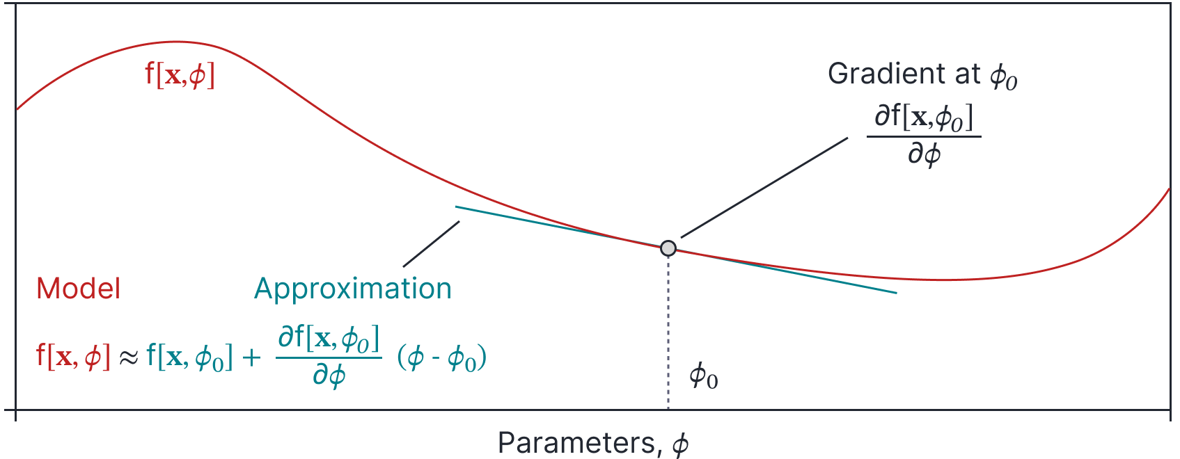
Figure 3. Taylor approximation. For a fixed input $\mathbf{x}$, the output $\mbox{f}[\mathbf{x},\boldsymbol\phi]$ of the model changes as a function of the choice of parameters $\boldsymbol\phi$ (orange curve). This relationship can be locally approximated by a linear function around initial parameters $\boldsymbol\phi_{0}$ (blue line), when the deviation from $\boldsymbol\phi_{0}$ is small.
Validity of linear approximation
The linear approximation will be valid if the curvature of $\mbox{f}[\mathbf{x},\boldsymbol\phi]$ with respect to the parameters $\boldsymbol\phi$ is small in the limited region that the parameters vary around $\boldsymbol\phi_{0}$ during training. More formally, Liu et al. (2020) identified that the spectral norm of the Hessian matrix containing the second derivatives must be small compared to the magnitude of the gradient in a ball of a certain radius.
Let’s show that this is true for a toy shallow network $\mbox{f}[x,\boldsymbol\phi]$ that maps scalar input $x$ to a scalar output:
\begin{equation}
\mbox{f}[x,\boldsymbol\phi] = \frac{1}{\sqrt{D}}\sum_{d=1}^{D} \theta_{d} \cdot \mbox{a}\bigl[\phi_{d}x\bigr],
\tag{7}
\end{equation}
where $a[\bullet]$ is a twice differentiable activation function. We’ll again assume that the weights $\theta_{d}$ that map from the hidden layer to the output are assigned randomly to $\pm 1$ and fixed, leaving just $D$ parameters $\phi_d$ that map from the input to the hidden layer. These are initialized from a standard normal distribution.
Hessian: For this model, the Hessian matrix $\mathbf{H}\in\mathbb{R}^{D\times D}$ is diagonal with values:
\begin{equation}
\mathbf{H}_{dd} = \frac{\partial^2 \mbox{f}[x,\boldsymbol\phi]}{\partial \phi^2_{d}} = \frac{1}{\sqrt{D}} \theta_{d}\mbox{a}^{”}\bigl[\phi_{d}x\bigr]x^2,
\tag{8}
\end{equation}
where $\mbox{a}^{”}[\bullet]$ is the second derivative of the activation function with respect to its inputs. If the input is bounded so $|x|\leq C$, then the spectral norm of the Hessian $\lVert \mathbf{H}\rVert$ is given by the maximum diagonal element:
\begin{eqnarray}
\bigl\lVert\mathbf{H} \bigr\rVert = \max_{d}\Bigl[\lVert\mathbf{H}_{dd}\rVert\Bigr] &=& \frac{x^2}{\sqrt{D}} \max_{d}\Bigl[\mbox{a}^{”}[\phi_d x]\Bigr] \nonumber \\
&\leq& \frac{C^2}{\sqrt{D}} \max_{d}\Bigl[\mbox{a}^{”}[\phi_d x]\Bigr]\nonumber \\
&\leq& \frac{C^2A}{\sqrt{D}}
\tag{9}
\end{eqnarray}
where $A$ is the maximum value of the second derivative $\mbox{a}^{”}[\bullet]$ of the activation function . It’s clear that as $D\rightarrow \infty$, the Hessian norm converges to zero.
Jacobian: Let’s compare that to what happens with the magnitude of the derivative vector:
\begin{eqnarray}
\sum_{d=1}^{D}\left(\frac{\partial \mbox{f}[x,\boldsymbol\phi]}{\partial \phi_d}\right)^2 = \frac{1}{D}\sum_{d=1}^{D} x^2\mbox{a}^{\prime}[\phi_{d}x],
\tag{10}
\end{eqnarray}
where the $\theta_d^2$ terms have disappeared as they equal one regardless of whether they were $\pm 1$. It’s easy to see that the magnitude of the gradient stays roughly constant as $D\rightarrow \infty$ because the factor $1/D$ cancels with the $D$ terms in the sum.
It follows that as the width $D$ increases, the curvature (Hessian) decreases, but the gradient (derivative vector) stays constant, and so the linear approximation is reasonable for this simple network when the width becomes very large. A more general proof for multi-layer networks with multiple inputs is provided by Liu et al. (2020).
Derivative vector as non-linear transformation
We have seen that as the hidden layers of neural networks become infinitely large:
- The change in any individual parameter from their initialized values during training decreases.
- The magnitude of the gradient of the function with respect to the parameter vector at initialization stays approximately constant.
- The second derivatives of the function with respect to the parameter vector at initialization decrease.
It follows that the network becomes approximately linear with respect to the parameters, and we can write:
\begin{equation}\label{eq:NTK_linear_approx}
\mathbf{ f}[\mathbf{x},\boldsymbol\phi] \approx \mathbf{ f }^{\ lin}[\mathbf{x},\boldsymbol\phi] = \mathbf{ f}[\mathbf{x},\boldsymbol\phi_0] + \frac{\partial \mathbf{ f}[\mathbf{x},\boldsymbol\phi_0]}{\partial \boldsymbol\phi}^T\bigl(\boldsymbol\phi-\boldsymbol\phi_{0}\bigr),
\tag{11}
\end{equation}
where $\mathbf{x}$ is an input example, and $\boldsymbol\phi_{0}$ is a vector containing all of the initial weights and biases.
One interpretation is that this expression is a linear function of a fixed non-linear transformation $\mathbf{ g}[\mathbf{x}]$ of the input $\mathbf{x}$:
\begin{eqnarray}
\mathbf{ f }^{\ lin}[\mathbf{x},\boldsymbol\phi] &=& \mathbf{ f}[\mathbf{x},\boldsymbol\phi_0] + \mathbf{ g}[\mathbf{x}]^T\bigl(\boldsymbol\phi-\boldsymbol\phi_{0}\bigr),
\tag{12}
\end{eqnarray}
where:
\begin{equation}
\mathbf{ g}[\mathbf{x}] = \frac{\partial \mathbf{f}[\mathbf{x},\boldsymbol\phi_0]}{\partial \boldsymbol\phi}.
\tag{13}
\end{equation}
This immediately brings to mind kernel methods which rely on dot products between nonlinear transformations $\mathbf{g}[\mathbf{x}_i]$ and $\mathbf{g}[\mathbf{x}_j]$ of input data examples $\mathbf{x}_{i},\mathbf{x}_{j}$. Hence, we now have all three components of the name neural tangent kernel. The term neural derives from neural networks, the term tangent from the first term in the Taylor expansion (see figure 3), and the term kernel from the interpretation of the gradient vector as a non-linear transformation of the input data.
Training dynamics
In the previous section, we saw that in the infinite width limit, the network predictions for an input $\mathbf{x}$ become a linear model with parameters $\boldsymbol\phi$. In part I of this series, we found closed-form expressions for the training dynamics for linear models. Now, we combine these observations to find closed-form expressions for the training dynamics of neural networks in the infinite limit.
For convenience, we will store all of the $I$ training data vectors $\{\mathbf{x}_{i}\}$ in the columns of a matrix $\mathbf{X}\in\mathbb{R}^{D\times I}$. We assume that the targets $\{y_{i}\}$ are scalar and store them in a column vector $\mathbf{y}\in\mathbb{R}^{I\times 1}$. A neural network model $\mathbf{f}[\mathbf{X},\boldsymbol\phi]$ is applied to all of the data simultaneously and produces an $I\times 1$ column vector whose $i^{th}$ entry is $\mbox{f}[\mathbf{x}_i,\boldsymbol\phi]$. The linear model can now be written as:
\begin{equation}\label{eq:NTK_linear_approx_all}
\mathbf{f }^{\ lin}[\mathbf{X},\boldsymbol\phi] = \mathbf{f}[\mathbf{X},\boldsymbol\phi_0] + \frac{\partial \mathbf{f}[\mathbf{X},\boldsymbol\phi_0]}{\partial \boldsymbol\phi}\bigl(\boldsymbol\phi-\boldsymbol\phi_{0}\bigr).
\tag{14}
\end{equation}
The derivative $\partial \mathbf{f}[\mathbf{X},\boldsymbol\phi_0]/\partial \boldsymbol\phi$ is an $I\times |\boldsymbol\phi|$ matrix containing derivatives for each of $I$ training examples and the $|\boldsymbol\phi|$ parameters.
In part I of this series, we showed that the ODE that governs the evolution of the residual differences between model predictions $\mathbf{f}[\mathbf{X},\boldsymbol\phi]$ and the ground truth targets $\mathbf{y}$ is:
\begin{eqnarray}\label{eq:NTK_r_ode}
\frac{d}{dt}\Bigl[\mathbf{f}[\mathbf{X},\boldsymbol\phi]-\mathbf{y}\Bigr] =-\left(\frac{\partial \mathbf{f}[\mathbf{X},\boldsymbol\phi]}{\partial \boldsymbol\phi} \frac{\partial \mathbf{f}[\mathbf{X},\boldsymbol\phi]}{\partial \boldsymbol\phi}^T\right)\Bigl(\mathbf{f}[\mathbf{X},\boldsymbol\phi]-\mathbf{y}\Bigr).
\tag{15}
\end{eqnarray}
For the linear approximation, the gradient terms only depend on the initial parameters $\boldsymbol\phi_{0}$ and so we can write:
\begin{eqnarray}\label{eq:NTK_r_ode2}
\frac{d}{dt}\Bigl[\mathbf{f}[\mathbf{X},\boldsymbol\phi]-\mathbf{y}\Bigr] =-\left(\frac{\partial \mathbf{f}[\mathbf{X},\boldsymbol\phi_0]}{\partial \boldsymbol\phi} \frac{\partial \mathbf{f}[\mathbf{X},\boldsymbol\phi_0]}{\partial \boldsymbol\phi}^T\right)\Bigl(\mathbf{f}[\mathbf{X},\boldsymbol\phi]-\mathbf{y}\Bigr),
\tag{16}
\end{eqnarray}
where we have dropped the superscript $lin$ for notational simplicity. This ODE has a closed form solution:
\begin{equation}\label{eq:NTK_r_ode3}
\mathbf{f}[\mathbf{X},\boldsymbol\phi_t]-\mathbf{y} = \exp\left[-\frac{\partial \mathbf{f}[\mathbf{X},\boldsymbol\phi_0]}{\partial \boldsymbol\phi} \frac{\partial \mathbf{f}[\mathbf{X},\boldsymbol\phi_0]}{\partial \boldsymbol\phi}^T\cdot t\right] \Bigl(\mathbf{f}[\mathbf{X},\boldsymbol\phi_0]-\mathbf{y}\Bigr).
\tag{17}
\end{equation}
The neural tangent kernel
We now refer to the $I\times I$ matrix from equation 17 as the neural tangent kernel or NTK for short:
\begin{equation}
\mathbf{NTK}\bigl[\mathbf{X},\mathbf{X}\bigr] = \frac{\partial \mathbf{f}[\mathbf{X},\boldsymbol\phi_0]}{\partial \boldsymbol\phi} \frac{\partial \mathbf{f}[\mathbf{X},\boldsymbol\phi_0]}{\partial \boldsymbol\phi}^T.
\tag{18}
\end{equation}
If we could compute this term, then we would have a closed-form solution for the evolution of the residuals, and the contents of this matrix would shine a light on the trainability and convergence speed of the system.
In principle could compute the NTK for a neural network by simply computing the derivatives for every training example $\mathbf{x}_{i}$ using the backpropagation algorithm and taking the appropriate dot products. However, it turns out that for some models, we can get a closed form solution for the NTK. The rest of this blog derives such solutions. Part III of this series returns to the implications of the neural tangent kernel.
Empirical NTK for a shallow network
Consider a shallow neural network with $D$ hidden units:
\begin{equation}
\mbox{f}[\mathbf{x},\boldsymbol\phi] = \frac{1}{\sqrt{D}} \sum_{d=1}^{D}\omega_{1d}\mbox{ a}\bigl[\boldsymbol\omega_{0d}\mathbf{x}\bigr],
\tag{19}
\end{equation}
where $\boldsymbol\omega_{0d}$ contains the weights that relate the input $\mathbf{x}$ to the $d^{th}$ hidden unit and $\omega_{1d}$ is the weight that relates $d^{th}$ hidden unit to the output. We have omitted the bias terms for simplicity.
The derivatives with regards to the two sets of parameters are:
\begin{eqnarray}
\frac{\partial \mbox{f}[\mathbf{x},\boldsymbol\phi]}{\partial\boldsymbol\omega_{0d}} &=& \frac{1}{\sqrt{D}}\sum_{d=1}^{D}\mbox{a}^{\prime}\bigl[\boldsymbol\omega_{0d}\mathbf{x}\bigr] \cdot \omega_{1d}\mathbf{x}\nonumber \\
\frac{\partial \mbox{f}[\mathbf{x},\boldsymbol\phi]}{\partial \omega_{1d}} &=& \frac{1}{\sqrt{D}} \mbox{a}\bigl[\boldsymbol\omega_{0d}\mathbf{x}\bigr].
\tag{20}
\end{eqnarray}
Since the inner product of the concatenated derivatives just the sum of the inner products of the individual derivatives, we can write a closed form expression for the kernel:
\begin{eqnarray}\label{eq:NTK_shallow_kernel_D}
\mbox{NTK}[\mathbf{x}_i,\mathbf{x}_{j}]&=& \sum_{d=1}^{D}\frac{\partial \mbox{f}[\mathbf{x}_i,\boldsymbol\phi]}{\partial\boldsymbol\omega_{0d}}\frac{\partial \mbox{f}[\mathbf{x}_j, \boldsymbol\phi]}{\partial\boldsymbol\omega_{0d}}+\frac{\partial \mbox{f}[\mathbf{x}_i,\boldsymbol\phi]}{\partial \omega_{1d}}\frac{\partial \mbox{f}[\mathbf{x}_j,\boldsymbol\phi]}{\partial \omega_{1d}} \\
&=& \frac{1}{D}\sum_{d=1}^{D}\omega_{1d}^2 \mbox{a}^{\prime}\bigl[\boldsymbol\omega_{0d}\mathbf{x}_i\bigr]\mbox{a}^{\prime}\bigl[\boldsymbol\omega_{0d}\mathbf{x}_j\bigr] \mathbf{x}_i^{T}\mathbf{x}_{j} +\mbox{a}\bigl[\boldsymbol\omega_{0d}\mathbf{x}_{i}\bigr] \mbox{a}\bigl[\boldsymbol\omega_{0d}\mathbf{x}_{j}\bigr]\nonumber.
\tag{21}
\end{eqnarray}
To make this concrete, let’s consider using the rectified linear unit (ReLU):
\begin{equation}\label{eq:snn_relu}
\mbox{a}[z] = \mbox{ReLU}[z] = \begin{cases} 0 & \quad z <0 \\ z & \quad z\geq 0\end{cases},
\tag{22}
\end{equation}
which has the derivative (figure 4):
\begin{equation}\label{eq:snn_relu2}
\mbox{a}^{\prime}[z] = \frac{d\mbox{ReLU}[z]}{dz} = \begin{cases} 0 & \quad z <0 \\ 1 & \quad z\geq 0\end{cases},
\tag{23}
\end{equation}
or $\mathbb{I}[z>0]$ for short. Here, the neural tangent kernel is given by:
\begin{eqnarray}\label{eq:NTK_empirical_kernel_}
\mbox{NTK}[\mathbf{x}_i,\mathbf{x}_{j}] &=& \frac{1}{D}\sum_{d=1}^{D}\omega_{1d}^2 \mathbb{I}\bigl[\boldsymbol\omega_{0d}\mathbf{x}_i > 0\bigr]\mathbb{I}\bigl[\boldsymbol\omega_{0d}\mathbf{x}_j > 0\bigr] \mathbf{x}_i^{T}\mathbf{x}_{j}\nonumber \\ &&\hspace{3cm} +\mbox{ReLU}\bigl[\boldsymbol\omega_{0d}\mathbf{x}_{i}\bigr] \mbox{ReLU}\bigl[\boldsymbol\omega_{0d}\mathbf{x}_{j}\bigr],
\tag{24}
\end{eqnarray}
where the first term is the component due to the derivatives in $\boldsymbol\omega_{0d}$ and the second term is the component due to the derivatives in $\boldsymbol\omega_{1}$. For finite width networks, the neural tangent kernel (however it was calculated) depends on the particular random draw of the parameters and here it’s referred to as the empirical tangent kernel.
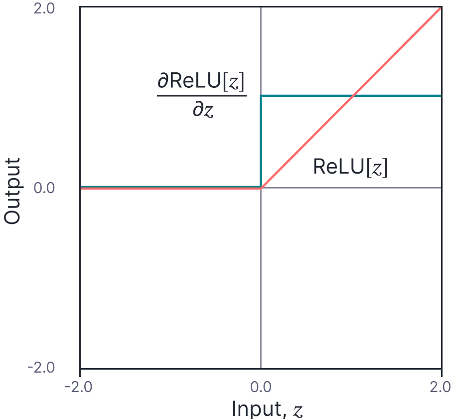
Figure 4. The rectified linear unit (ReLU) activation function. The ReLU function (orange line) returns zero when the input is less than zero, or the input itself otherwise. It’s derivative (cyan line) is zero when the input is less than zero and one otherwise. Adapted from $\href{http://udlbook.com}{\color{blue}Prince (2023)}$.
Analytical NTK for shallow network
If we let the number of hidden units $D\rightarrow \infty$, then the summation in equation 29 becomes an expectation over the contributions of the hidden units and we have:
\begin{eqnarray}
\mbox{NTK}[\mathbf{x}_i,\mathbf{x}_{j}]&=&\ \\
&&\hspace{-1cm}\mathbb{E}_{\boldsymbol\omega_0,\boldsymbol\omega_1}\biggl[\boldsymbol\omega_{1}^2 \mathbb{I}\bigl[\boldsymbol\omega_{0}\mathbf{x}_i > 0\bigr]\mathbb{I}\bigl[\boldsymbol\omega_{0}\mathbf{x}_j > 0\bigr] \mathbf{x}_i^{T}\mathbf{x}_{j} +\mbox{ReLU}\bigl[\boldsymbol\omega_{0}\mathbf{x}_{i}\bigr] \mbox{ReLU}\bigl[\boldsymbol\omega_{0}\mathbf{x}_{j}\bigr]\biggr].\nonumber
\tag{25}
\end{eqnarray}
For variables $\mathbf{z}=[z_{i},z_{j}]^T$ with mean $\mathbf{0}$ and covariance:
\begin{equation}
\boldsymbol\Sigma = \begin{bmatrix}\sigma_{i}^2 & \sigma_{ij}^2 \\ \sigma_{ij}^2 & \sigma_{j}^2\end{bmatrix},
\tag{26}
\end{equation}
it can (non-obviously) be shown that that
\begin{eqnarray}
\mathbb{E}\Bigl[\mbox{ReLU}[z_{i}]]\cdot \mbox{ReLU}[z_{j}]\Bigr]
&=& \frac{\sigma_{i}\sigma_j\Bigl(\cos[\theta]\cdot \Bigl(\pi -\theta\Bigr)+\sin[\theta]\Bigr)}{2\pi}\nonumber \\
\mathbb{E}\Bigl[\mathbb{I}[z_{i}>0]\cdot \mathbb{I}[z_{j}>0]\Bigr]
&=& \frac{\pi-\theta}{2\pi}
\tag{27}
\end{eqnarray}
where
\begin{equation}
\theta = \arccos\left[\frac{\sigma^2_{ij}}{\sigma_i\cdot\sigma_j}\right].
\tag{28}
\end{equation}
See Cho and Saul, 2009 and Golikov et al. (2022) for full proofs.
Assuming that both sets of weights are initialized from a standard normal distribution, we have $\sigma_{i}=|\mathbf{x}_{i}|, \sigma_{j}=|\mathbf{x}_{j}|$, and $\sigma_{ij} = \mathbf{x}_{i}^{T}\mathbf{x}_{j}$ which gives the final result:
\begin{eqnarray}\label{eq:NTK_shallow_kernel_D2}
\mbox{NTK}[\mathbf{x}_i,\mathbf{x}_{j}]&=& \frac{\mathbf{x}_{i}^{T}\mathbf{x}_{j}}{2\pi}(\pi-\theta) + \frac{|\mathbf{x}_{i}|\cdot |\mathbf{x}_{j}|}{2\pi} \Bigl((\pi-\theta)\cos[\theta] +\sin[\theta] \Bigr).
\tag{29}
\end{eqnarray}
Note that in the infinite limit, the kernel is constant; it does not depend on the initial choices for the parameters. We term this the analytical kernel. This result can be extended to deep neural networks where the kernel at each layer is computed as a function of the kernel at the previous layer (see following section). The analytical NTK also been calculated for convolutional networks (Arora et al., 2019, Li et al. 2019) and other common architectures.
Empirical NTK for a deep network
We can similarly compute the NTK for a deep network. Here, the NTK is computed iteratively, by expressing the NTK for a depth $L$ network in terms of the NTK for a depth $L-1$ network. This section derives this result. It is rather mathematically involved and can be skipped on the first reading. It is not required to understand part III of this blog.
Linear model, one output
We start with a linear model $\mbox{f}_0[\mathbf{x},\boldsymbol\phi_0]$ (figure 5):
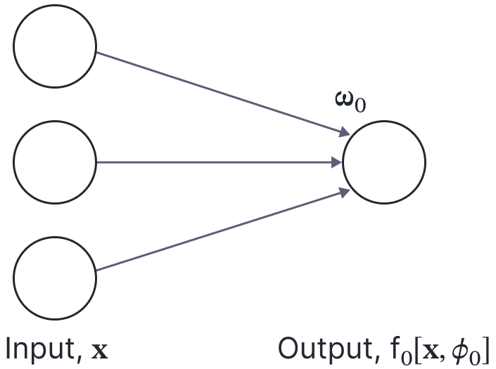
Figure 5. Building up the NTK computation for a deep neural network. We first consider a linear model $\mbox{f}_0[\mathbf{x},\boldsymbol\phi_{0}]$ with one output, bias $\beta_{0}$ (not shown), and weights $\boldsymbol\omega_0$.
\begin{equation}
\mbox{f}_0\left[\mathbf{x},\boldsymbol\phi_0\right] = \beta_0 + \frac{1}{\sqrt{D_{in}}} \boldsymbol\omega_0\mathbf{x},
\tag{30}
\end{equation}
where $D_{in}$ is the input data dimension and the parameters $\boldsymbol\phi_{0} =\{\beta_0,\boldsymbol\omega_0\}$ comprise the bias $\beta_{0}\in\mathbb{R}$ and the weights $\boldsymbol\omega_{0}\in\mathbb{R}^{1\times D_{in}}$. The value of the NTK at position $(i,j)$ is:
\begin{eqnarray}
\mbox{NTK}[\mathbf{x}_i,\mathbf{x}_j] &=& \frac{\partial \mbox{f}[\mathbf{x}_i,\boldsymbol\phi_0]}{\partial \boldsymbol\phi_0}^{T}\frac{\partial \mbox{f}[\mathbf{x}_j,\boldsymbol\phi_0]}{\partial \boldsymbol\phi_0}\nonumber \\
&=& \frac{\partial \mbox{f}[\mathbf{x}_i,\boldsymbol\phi_0]}{\partial \boldsymbol\omega_0}^{T}\frac{\partial \mbox{f}[\mathbf{x}_j,\boldsymbol\phi_0]}{\partial \boldsymbol\omega_0} + \frac{\partial \mbox{f}[\mathbf{x}_i,\boldsymbol\phi_0]}{\partial \beta_0}^{T}\frac{\partial \mbox{f}[\mathbf{x}_j,\boldsymbol\phi_0]}{\partial \beta_0}\nonumber\\
&=& \frac{1}{D_{in}}\mathbf{x}_i^T\mathbf{x}_j+1.
\tag{31}
\end{eqnarray}
Linear model, D outputs
Now consider a linear model $\mathbf{f}_0[\mathbf{x},\boldsymbol\phi_0]$ with $D$ outputs (figure 6):

Figure 6. Building up the NTK computation for a deep neural network. Now we consider a linear model $\mathbf{f}_0[\mathbf{x},\boldsymbol\phi_{0}]$ with $d$ outputs, biases $\beta_{0,d}$ (not shown) and weights $\boldsymbol\omega_{0,d}$.
\begin{equation}
\mbox{f}_{0,d}\left[\mathbf{x},\boldsymbol\phi_0\right] = \beta_{0,d} + \frac{1}{\sqrt{D_{in}}} \boldsymbol\omega_{0,d}\mathbf{x},
\tag{32}
\end{equation}
where $\beta_{0,d}\in\mathbb{R}$ and $\boldsymbol\omega_{0,d}\in\mathbb{R}^{1\times D_{in}}$. The neural tangent kernel now has $ID\times ID$ elements which correspond to the dot product of the gradients for every pair of the $I$ input vectors and $D$ outputs. It is arranged to form $I\times I$ sub-kernels $\mathbf{NTK}[\mathbf{x}_{i},\mathbf{x}_{j}]$ each of size $D\times D$ and containing sub-elements $\mbox{NTK}_{d,d’}[\mathbf{x}_i,\mathbf{x}_j]$ (figure 7). By the same logic as the previous section each has the same value:
\begin{eqnarray}\label{eq:NTK_linear_kernel}
\mbox{NTK}_{d,d’}[\mathbf{x}_i,\mathbf{x}_j] = \frac{1}{D_{in}}\mathbf{x}_i^T\mathbf{x}_j+1.
\tag{33}
\end{eqnarray}
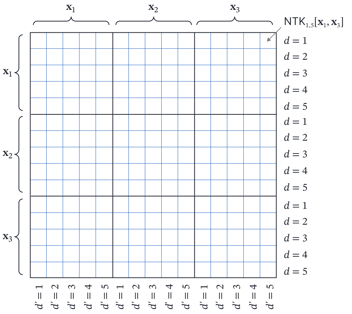
Figure 7. Kernel structure for linear model with $D$ outputs. For $I$ inputs, the kernel matrix now consists of $I\times I$ subkernels, each of size $D\times D$.
Fully connected network with one layer
Next, we consider a fully connected network $\mbox{f}_{1}[\mathbf{x},\boldsymbol\phi_1]$ with a single output and one hidden layer containing $D$ neurons, associated parameters $\boldsymbol\phi_1 =\{\boldsymbol\beta_0,\boldsymbol\Omega_0,\beta_1,\boldsymbol\omega_1\}$ and activation function $\mathbf{a}[\bullet]$ (figure 8):
\begin{equation}
\mbox{f}_{1}\left[\mathbf{x},\boldsymbol\phi_1\right] = \beta_1+ \frac{1}{\sqrt{D}} \boldsymbol\omega_{1}\mathbf{a}\Bigl[\mathbf{f}_{0}\left[\mathbf{x},\boldsymbol\phi_0\right]\Bigr],
\tag{34}
\end{equation}

Figure 8. Building up the NTK computation for a deep neural network. We pass each of the outputs from figure 6 through an activation function $\mathbf{a}[\bullet]$ and recombine using bias $\beta_{1,1}$ (not shown) and weights $\boldsymbol\omega_{1}$ to create a neural network $\mathbf{f}[\mathbf{x},\boldsymbol\phi_{1}]$ with a single hidden layer.
where the preactivation $\mbox{f}_{0,d}\left[\mathbf{x},\boldsymbol\phi_0\right]~$ at each hidden unit is the linear function discussed above:
\begin{equation}
\mbox{f}_{0,d}\left[\mathbf{x},\boldsymbol\phi_0\right] = \beta_{d} + \frac{1}{\sqrt{D_{in}}} \boldsymbol\omega_{0d}\mathbf{x},
\tag{35}
\end{equation}
and $\boldsymbol\phi_{0}=\{\beta_{0,1}\ldots \beta_{0,D_{in}}, \boldsymbol\omega_{0,1}\ldots \boldsymbol\omega_{0,D_{in}}\}$.
The derivatives of $\mbox{f}_{1}[\mathbf{x},\boldsymbol\phi_1]$ with respect to the unknown quantities are:
\begin{eqnarray}\label{eq:NTK_deep_derivs}
\frac{\partial \mbox{f}_{1}\left[\mathbf{x},\boldsymbol\phi_1\right]}{\partial \boldsymbol\omega_{1}} &=& \frac{1}{\sqrt{D}} \mathbf{a}\Bigl[\mathbf{f}_{0}\left[\mathbf{x},\boldsymbol\phi_0\right]\Bigr] \nonumber \\
\frac{\partial\mbox{f}_{1}\left[\mathbf{x},\boldsymbol\phi_1\right]}{\partial \beta_{1}} &=& 1 \nonumber \\
\frac{\partial\mbox{f}_{1}\left[\mathbf{x},\boldsymbol\phi_1\right]}{\partial \boldsymbol\phi_0} &=& \frac{1}{\sqrt{D}}\biggl(\bf1\mathbf{a}’\Bigl[\mathbf{f}_0\left[\mathbf{x},\boldsymbol\phi_0\right]\Bigr]^T\odot\frac{\partial \mathbf{f}_{0}\left[\mathbf{x},\boldsymbol\phi_0\right]}{\partial \boldsymbol\phi_0}\biggr)\boldsymbol\omega_{1}^T,
\tag{36}
\end{eqnarray}
where $\partial \mathbf{f}_{0}\left[\mathbf{x},\boldsymbol\phi_0\right]/\partial \boldsymbol\phi_0$ is a $|\boldsymbol\phi_0|\times D$ matrix which is block diagonal since only $D_{in}$ weights and one bias in $\boldsymbol\phi_0$ modify any particular element of the activation vector. The term $\bf1$ is a $|\boldsymbol\phi|\times 1$ column vector containing only ones, and $\odot$ represents pointwise multiplication.
Now we compute the elements $\mbox{NTK}^{(1)}[\mathbf{x}_i,\mathbf{x}_j]$ of the kernel for this shallow network by taking the dot products of the derivatives with respect to the parameters:
\begin{eqnarray}
\mathbf{NTK}^{(1)}[\mathbf{x}_i,\mathbf{x}_j]
&=&\frac{\partial \mbox{f}_{1}\left[\mathbf{x}_i,\boldsymbol\phi_1\right]}{\partial \boldsymbol\omega_1}^{T}\frac{\partial \mbox{f}_{1}\left[\mathbf{x}_j,\boldsymbol\phi_1\right]}{\partial \boldsymbol\omega_1} + \frac{\partial \mbox{f}_{1}\left[\mathbf{x}_i,\boldsymbol\phi_1\right]}{\partial \beta_1}^{T}\frac{\partial \mbox{f}_{1}\left[\mathbf{x}_j,\boldsymbol\phi_1\right]}{\partial \beta_1}
\nonumber \\
&&\hspace{3.76cm}+\frac{\partial \mbox{f}_{1}\left[\mathbf{x}_i,\boldsymbol\phi_1\right]}{\partial \boldsymbol\phi_0}^{T}\frac{\partial \mbox{f}_{1}\left[\mathbf{x}_j,\boldsymbol\phi_1\right]}{\partial \boldsymbol\phi_0}.
\tag{37}
\end{eqnarray}
Substituting in the derivatives from equation 36, we see that:
\begin{eqnarray}
\mathbf{NTK}^{(1)}[\mathbf{x}_i,\mathbf{x}_j] &=& \tag{38}\\ &&\hspace{-2.8cm}\frac{1}{D}\Biggl(\mathbf{a}\Bigl[\mathbf{f}_{0}\left[\mathbf{x}_i,\boldsymbol\phi_0\right]\Bigr]^T \mathbf{a}\Bigl[\mathbf{f}_{0}\left[\mathbf{x}_j,\boldsymbol\phi_0\right]\Bigr] +D\\
&&\hspace{-2.5cm}+\hspace{0.1cm}\boldsymbol\omega_1\Biggl(\mathbf{a}’\Bigl[\mathbf{f}_0\left[\mathbf{x}_i,\boldsymbol\phi_0\right]\Bigr]\mathbf{a}’\Bigl[\mathbf{f}_0\left[\mathbf{x}_j,\boldsymbol\phi_0\right]\Bigr]^T\odot\frac{\partial \mathbf{f}_{0}\left[\mathbf{x}_i,\boldsymbol\phi_0\right]}{\partial \boldsymbol\phi_0}^T\frac{\partial \mathbf{f}_{0}\left[\mathbf{x}_j,\boldsymbol\phi_0\right]}{\partial \boldsymbol\phi_0}\Biggr)\boldsymbol\omega_{1}^T\Biggr).\nonumber
\end{eqnarray}
and noting that the product of the derivative terms is just the neural tangent kernel $\mathbf{NTK}^{(0)}[\mathbf{x}_{i},\mathbf{x}_{j}]$ from the single layer network, we see that:
\begin{eqnarray}
\mathbf{NTK}^{(1)}[\mathbf{x}_i,\mathbf{x}_j] \!\!&\!\!=\!\!&\!\!
\frac{1}{D}\Biggl(\mathbf{a}\Bigl[\mathbf{f}_{0}\left[\mathbf{x}_i,\boldsymbol\phi_0\right]\Bigr]^T \mathbf{a}\Bigl[\mathbf{f}_{0}\left[\mathbf{x}_j,\boldsymbol\phi_0\right]\Bigr] +D \\
&&\hspace{-0.0cm}+\hspace{0.1cm}\boldsymbol\omega_1\Biggl(\mathbf{a}’\Bigl[\mathbf{f}_0\left[\mathbf{x}_i,\boldsymbol\phi_0\right]\Bigr]\mathbf{a}’\Bigl[\mathbf{f}_0\left[\mathbf{x}_j,\boldsymbol\phi_0\right]\Bigr]^T\odot \mathbf{NTK}^{(0)}[\mathbf{x}_{i},\mathbf{x}_{j}]\Biggr)\boldsymbol\omega_{1}^T\Biggr).\nonumber
\tag{39}
\end{eqnarray}
Hence, the NTK for the network with one hidden layer can be written in terms of the NTK for a network with no hidden layers.
Recursive calculation of kernel
In the previous equation, we the kernel $\mathbf{NTK}^{(1)}[\mathbf{x}_i,\mathbf{x}_j]$ associated with the single output of a shallow network in terms of the $D\times D$ subkernel $\mathbf{NTK}~^{(0)}[\mathbf{x}_{i},\mathbf{x}_{j}]$ of the preactivations. As might be expected, there is a general formula that relates the kernel values at layer $l$ to those at layer $l-1$:
\begin{eqnarray}\label{eq:NTK_multilayer_final}
\mbox{NTK}^{(0)}_{d,d’}[\mathbf{x}_i,\mathbf{x}_j] &=&
\frac{1}{D_{in}}\mathbf{x}_i^T\mathbf{x}_j+1\\
\mbox{NTK}^{(l)}_{d,d’}[\mathbf{x}_i,\mathbf{x}_j] &=& \frac{1}{D}\Biggl(\mathbf{a}\Bigl[\mathbf{f}_{l-1}\left[\mathbf{x}_i,\boldsymbol\phi_{l-1}\right]\Bigr]^T \mathbf{a}\Bigl[\mathbf{f}_{l-1}\left[\mathbf{x}_j,\boldsymbol\phi_{l-1}\right]\Bigr] +D\nonumber \\
&&\hspace{-1.5cm}+\hspace{0.1cm}\boldsymbol\omega_{ld}\Biggl(\mathbf{a}’\Bigl[\mathbf{f}_{l-1}\left[\mathbf{x}_i,\boldsymbol\phi_{l-1}\right]\Bigr]\mathbf{a}’\Bigl[\mathbf{f}_{l-1}\left[\mathbf{x}_j,\boldsymbol\phi_{l-1}\right]\Bigr]^T\odot \mathbf{NTK}^{(l-1)}[\mathbf{x}_{i},\mathbf{x}_{j}]\Biggr)\boldsymbol\omega_{ld’}^T\Biggr).\nonumber
\tag{40}
\end{eqnarray}
We can use this recursive formulation to calculate the kernel for networks of arbitrary depth (figure 9).
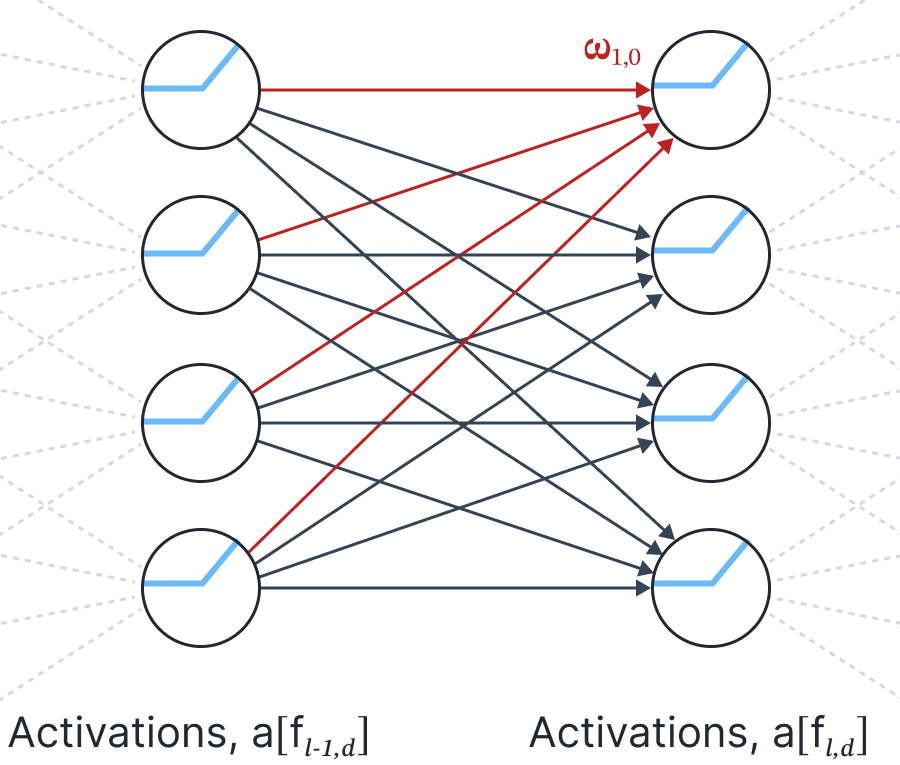
Figure 9. Building up the NTK computation for a deep neural network. Finally, we consider the general relationship between the NTK at layer $l$ and layer $l-1$ of a deep network.
Analytical NTK for deep network
To compute the analytical NTK, we let the number of hidden units in each dimension become infinite. Then the sums that are implicit in the vector operations in equation 41 become expectations and we have:
\begin{eqnarray}\label{eq:NTK_multilayer_final2}
\mbox{NTK}^{(0)}_{d,d’}[\mathbf{x}_i,\mathbf{x}_j] &=&
\frac{1}{D_{in}}\mathbf{x}_i^T\mathbf{x}_j+1\\
\mbox{NTK}^{(l)}_{d,d’}[\mathbf{x}_i,\mathbf{x}_j] &=& \mathbf{K}_{l}[\mathbf{x},\mathbf{x}’] +1+ \mathbf{K}_{l}'[\mathbf{x}_i,\mathbf{x}_{j}] \odot \mathbf{NTK}^{(l-1)}[\mathbf{x}_{i},\mathbf{x}_{j}],\nonumber
\tag{41}
\end{eqnarray}
where:
\begin{eqnarray}\label{eq:NTK_multilayer_final3}
\mathbf{K}_{0}[\mathbf{x}_{i},\mathbf{x}_{j}] &=& \mathbf{x}_{i}\mathbf{x}_{j}^T+1\\
\mathbf{K}’_{0}[\mathbf{x}_{i},\mathbf{x}_{j}] &=& \mathbf{x}_{i}\mathbf{x}_{j}^T+1\nonumber \\
\mathbf{K}_{l}[\mathbf{x}_{i},\mathbf{x}_{j}] &=& \mathbb{E}_{\mbox{f}_{l-1}\sim \mbox{Norm}[\mathbf{0},\mathbf{K}_{l-1}]}
\biggl[\mathbf{a}\Bigl[\mathbf{f}_{l-1}\left[\mathbf{x}_i,\boldsymbol\phi_{l-1}\right]\Bigr]^T \mathbf{a}\Bigl[\mbox{f}_{l-1,d}\left[\mathbf{x}_j,\boldsymbol\phi_{l-1}\right]\Bigr]\biggr],\nonumber \\
\mathbf{K}’_{l}[\mathbf{x}_{i},\mathbf{x}_{j}] &=& \mathbb{E}_{\mbox{f}_{l-1}\sim \mbox{Norm}[\mathbf{0},\mathbf{K}_{l-1}]}
\biggl[\mathbf{a}’\Bigl[\mathbf{f}_{l-1}\left[\mathbf{x}_i,\boldsymbol\phi_{l-1}\right]\Bigr]^T \mathbf{a}’\Bigl[\mbox{f}_{l-1,d}\left[\mathbf{x}_j,\boldsymbol\phi_{l-1}\right]\Bigr]\biggr].\nonumber
\tag{42}
\end{eqnarray}
Analytical NTK for deep ReLU network
Let’s assume that we use a ReLU for the activation functions. Here the derivative is $a'[z] =\mathbb{I}[z>0]$, and we can again use the results that for expectations taken with respect to a normal distribution with mean zero and covariance:
\begin{equation}
\boldsymbol\Sigma = \begin{bmatrix}
\sigma^{2}_i &\sigma^{2}_{ij} \\ \sigma^{2}_{ij} & \sigma^2_{i},
\end{bmatrix}
\tag{43}
\end{equation}
we have:
\begin{eqnarray}
\mathbb{E}_{\mbox{f}_{l-1}\sim \mbox{Norm}[\mathbf{0},\boldsymbol\Sigma]}\Bigl[\mbox{ReLU}[z_{i}]]\cdot \mbox{ReLU}[z_{j}]\Bigr]
&=& \frac{\sigma_{i}\sigma_j\Bigl(\cos[\theta]\cdot \Bigl(\pi -\theta\Bigr)+\sin[\theta]\Bigr)}{2\pi}\nonumber \\
\mathbb{E}_{\mbox{f}_{l-1}\sim \mbox{Norm}[\mathbf{0},\boldsymbol\Sigma]}\Bigl[\mathbb{I}[z_{i}>0]\cdot \mathbb{I}[z_{j}>0]\Bigr]
&=& \frac{\pi-\theta}{2\pi},
\tag{44}
\end{eqnarray}
where
\begin{equation}
\theta = \arccos\left[\frac{\sigma^2_{ij}}{\sigma_i\cdot\sigma_j}\right].
\tag{45}
\end{equation}
A cursory inspection of these equations reveals that substituting these results into the recursive formulae in equations 41-42 with $L=1$ yields the NTK for a shallow ReLU network that we derived in equation 29.
Conclusion
This blog has argued that when neural networks become very wide, their parameters do not change much during training and they can be considered as approximately linear. This linearity means that we can write a closed form solution for the training dynamics, and this closed form solution depends critically on the neural tangent kernel. Each element of the neural tangent kernel consists of the inner product of the vectors of derivatives for a pair of training data examples. This can be calculated for any network and we call this the empirical NTK. If we let the width become infinite, then we can get closed-form solutions, which are referred to as analytical NTKs. We derived these solutions for both shallow and deep ReLU networks. Part III of this series of blogs will investigate the implications of the neural tangent kernel.
How to Join The RBC Borealis Team!
Are you aspiring to build a career in AI and ML research? Do you want to join a team that is associated with innovation and high ethical standards? If you are looking for opportunities to make a personal impact, we have several programs and opportunities.
View open roles