
This blog is the fourth in a series in which we consider machine learning from four different viewpoints. We either use gradient descent or a fully Bayesian approach and for each, we can choose to focus on either the model parameters or the output function (figure 1). In part I, we considered gradient descent with infinitesimal steps (gradient flow) for linear models with a least squares loss. This provided insights into both how the parameters and the output function evolve over time during training. In part II and part III, we explored gradient flow in deep neural networks and this led to the development of the neural tangent kernel.
The following articles in this series follow a similar structure. In this blog (part IV) we investigate Bayesian methods for linear models with a least squares loss. We first consider the parameter space perspective. Here, we no longer aim to find the best set of parameters, but instead compute a probability distribution over possible parameter values and take into account all of these possible values when we make predictions. In part V then consider the output function perspective. Here, we treat the training and test points as jointly distributed as a Gaussian (i.e., a Gaussian process) and exploit this to make new predictions. In part VI and part VII, we will apply these ideas to deep neural networks, leading to Bayesian neural networks (parameter space) and neural network Gaussian processes (function space).
This article is accompanied by example Python code.
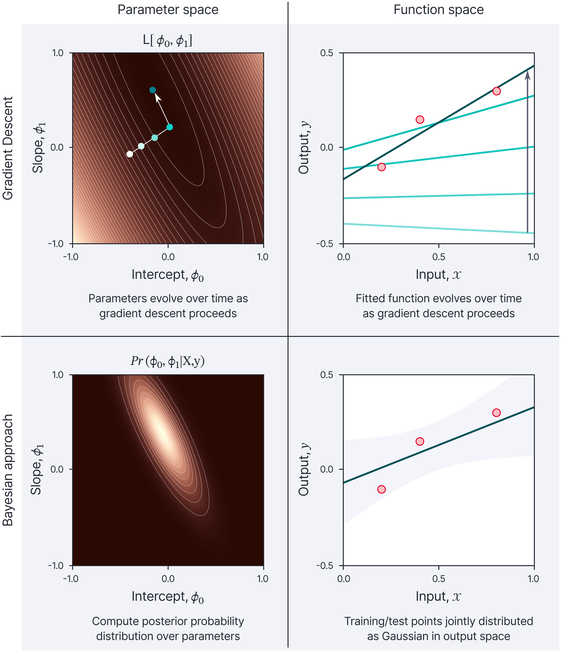
Figure 1. Four approaches to model fitting. We can either consider gradient descent (top row) or the Bayesian approach (bottom row). For either, we can consider either parameter space (left column) or the function space (right column). This blog concerns the Bayesian approach in parameter space (lower-left panel). Part V of this series will consider the Bayesian approach in function space (lower-right panel). Figure inspired by Sohl-Dickstein (2021).
Parameter space
In the maximum likelihood approach, we establish the best model parameters by finding the minimum of the loss function using gradient descent (or a closed-form solution if available). To motivate Bayesian methods, we draw attention to three potential disadvantages of this scheme. First, we do not take account of any prior information we have about the parameter values. Second, the final choice of parameters may be somewhat arbitrary; there may be many parameter values that fit the data reasonably well, but which extrapolate from that data quite differently (figure 2). Third, we do not get an estimate of uncertainty; intuitively, we expect our predictions to be less certain when they are far from the training points.
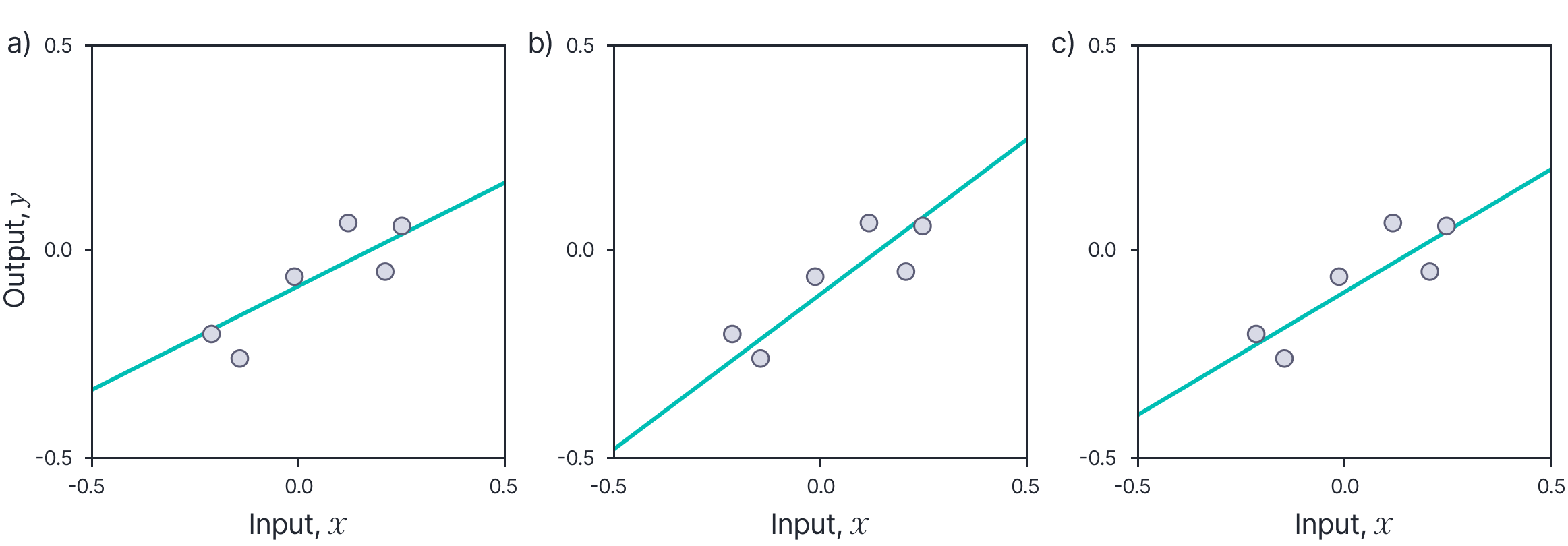
Figure 2. Drawback of maximum likelihood fitting. a) This line is a reasonable fit to the data. b) However, this line with a different slope and intercept is also a plausible description, as is c) this third line. The observed noisy data does not really allow us to distinguish which of these models is correct. It is hence worrying that the predictions of the three models when they extrapolate to $x=-0.5$ or $x=0.5$, are quite different. Maximum likelihood inherently commits to one “best” set of parameters and ignores the fact that there may be many other parameter settings that are almost as good, but which extrapolate from the data quite differently.
Overview of the Bayesian approach
The Bayesian approach rejects the idea that we should find a single set of parameters. Instead, it treats all parameter values as possible but acknowledges that some are more probable than others depending on the degree to which they are compatible with the noisy data; rather than finding a single set of parameter values, the Bayesian approach finds a probability distribution over possible parameters in the training process.
This complicates inference (predicting the model output for a new input). We cannot just run the model straightforwardly as there is no single set of parameters. Instead, we make separate predictions for each possible set of parameter values and take a weighted average of these predictions, where the weight is given by the probability of those parameters as established from the training data.
From maximum likelihood to the Bayesian approach
In this section, we make these ideas concrete for an arbitrary model $y=\mathrm{f}[\mathbf{x}, \boldsymbol{\phi}]$ which takes a multivariate input $\mathbf{x}$ and returns a single scalar output $y$ and has parameters $\boldsymbol{\phi}$. We assume that we are given a training dataset $\left\{\mathbf{x}_{i}, y_{i}\right\}_{i=1}^{I}$ containing $I$ input-output pairs, and that we have a noise model $\operatorname{Pr}\left(y_{i} \mid \mathbf{x}_{i}, \boldsymbol{\phi}\right)$ which specifies how likely we are to observe the training output $y_{i}$ given input $\mathbf{x}_{i}$ and model parameters $\boldsymbol\phi$. For a regression problem, this would typically be a normal distribution where the mean is specified by the model output, and the noise variance $\sigma_{n}^{2}$ is constant:
\begin{equation*}
\operatorname{Pr}\left(y_{i} \mid \mathbf{x}_{i}, \boldsymbol{\phi}\right)=\operatorname{Norm}_{y_{i}}\left[\mathrm{f}\left[\mathbf{x}_{i}, \boldsymbol{\phi}\right], \sigma_{n}^{2}\right]. \tag{1}
\end{equation*}
For different types of problems like classification or ranking, the noise model would differ.
Maximum likelihood approach
As the name suggests, the maximum likelihood approach finds the parameters $\hat{\boldsymbol\phi}$ that maximize the likelihood of the training data, assuming that the inputs are independent and identically distributed:
\begin{equation*}
\hat{\boldsymbol\phi}_{ML}=\operatorname{argmax}\left[\prod_{i=1}^{I} \operatorname{Pr}\left(y_{i} \mid \mathbf{x}_{i}, \boldsymbol{\phi}\right)\right]. \tag{2}
\end{equation*}
To perform inference for a new input $\mathbf{x}^{*}$ we simply run the model $y^{*}=\mathrm{f}[\mathbf{x}^{*}, \hat{\boldsymbol{\phi}}]$ with the estimated parameters $\hat{\boldsymbol\phi}$.
Maximum a posteriori approach
We can easily extend this model to incorporate prior information about the parameters $\boldsymbol\phi$ by defining a prior probability distribution $\operatorname{Pr}(\boldsymbol\phi)$. This reflects what we know about the parameters of the model before we observe the data. This might be nothing (implying that $\operatorname{Pr}(\boldsymbol\phi)$ is uniform) or might reflect a generic preference for some types of input/output relation. A common choice is to favor parameter values with small magnitudes over those with large magnitudes. In neural networks, this encourages models where the output changes slowly as a function of the input. We modify our training criterion to incorporate the prior:
\begin{equation*}
\hat{\boldsymbol\phi}_{M A P}=\operatorname{argmax}\left[\prod_{i=1}^{I} \operatorname{Pr}\left(y_{i} \mid \mathbf{x}_{i}, \boldsymbol{\phi}\right) \operatorname{Pr}(\boldsymbol{\phi})\right]. \tag{3}
\end{equation*}
This is known as the maximum a posteriori or MAP approach.
Bayesian approach
In the Bayesian approach, we apply Bayes’ rule to find a distribution over the parameters:
\begin{equation*}
\operatorname{Pr}\left(\boldsymbol{\phi} \mid\left\{\mathbf{x}_{i}, \mathbf{y}_{i}\right\}\right)=\frac{\prod_{i=1}^{I} \operatorname{Pr}\left(y_{i} \mid \mathbf{x}_{i}, \boldsymbol{\phi}\right) \operatorname{Pr}(\boldsymbol{\phi})}{\int \prod_{i=1}^{I} \operatorname{Pr}\left(y_{i} \mid \mathbf{x}_{i}, \boldsymbol{\phi}\right) \operatorname{Pr}(\boldsymbol{\phi}) d \boldsymbol{\phi}}. \tag{4}
\end{equation*}
The left-hand side is referred to as the posterior probability of the parameters, which takes into account both the likelihood $\prod_{i} \operatorname{Pr}\left(y_{i} \mid \mathbf{x}_{i}, \boldsymbol\phi\right)$ of the parameters given the observed data, and the prior information about the parameters $\operatorname{Pr}(\boldsymbol{\phi})$. The posterior probability will be high for values that are both compatible with the data and have a high prior probability. For example, the parameters associated with all three lines in figure 2 might all have a high posterior probability.
As an aside, note that it is now easy to understand the term maximum a posteriori inference. Equation 3 maximizes the numerator of the right-hand side of equation 4 with respect to the parameters $\boldsymbol\phi$. Since the denominator does not depend on the parameters $\boldsymbol\phi$ (they are integrated out), this is equivalent to maximizing the left-hand side (i.e., finding the maximum of the posterior probability).
Returning to the Bayesian approach, we are now faced with the problem of how to perform inference (compute the estimate $\hat{y}^{*}$ for a new input $\mathbf{x}^{*}$). This is no longer straightforward, since we do not have a single estimate of the parameters, but a posterior distribution over possible parameters. The solution is to marginalize over (integrate over) the uncertain parameters $\boldsymbol\phi$:
\begin{equation*}
\operatorname{Pr}\left(y^{*} \mid \mathbf{x}^{*},\left\{\mathbf{x}_{i}, \mathbf{y}_{i}\right\}\right)=\int \operatorname{Pr}\left(y^{*} \mid \mathbf{x}^{*}, \boldsymbol{\phi}\right) \operatorname{Pr}\left(\boldsymbol{\phi} \mid\left\{\mathbf{x}_{i}, \mathbf{y}_{i}\right\}\right) d \boldsymbol{\phi} . \tag{5}
\end{equation*}
This can be interpreted as weighting together the predictions of an infinitely large ensemble of models (via the integral), where there is one model $\operatorname{Pr}\left(y^{*} \mid \mathbf{x}^{*}, \boldsymbol{\phi}\right)$ for each choice of parameters $\boldsymbol\phi$. The weight for that model is given by the associated posterior probability $\operatorname{Pr}\left(\boldsymbol\phi \mid\left\{\mathbf{x}_{i}, \mathbf{y}_{i}\right\}\right)$ (i.e., a measure of how compatible it was with the training data).
Example: linear model
Let’s put these ideas into practice using a linear regression model $y=\mathrm{f}[\mathbf{x}, \boldsymbol{\phi}]$ which takes a multivariate input $\mathbf{x} \in \mathbb{R}^{D}$ and computes a single scalar output $y$ and has the form:
\begin{equation*}
\mathrm{f}[\mathbf{x}, \boldsymbol{\phi}]=\mathbf{x}^{T} \boldsymbol{\phi}, \tag{6}
\end{equation*}
where $\boldsymbol\phi \in \mathbb{R}^{D}$ are the model parameters. We can extend this to an affine model by setting $\mathbf{x} \leftarrow\left[\begin{array}{lll}1 & \mathbf{x}^{T}\end{array}\right]^{T}$ (i.e., inserting the value 1 at the start of the input vector), where now the first value of $\boldsymbol\phi$ controls the $y$-offset of the model. For convenience, and according to the usual convention in machine learning, we will still refer to this as a linear model.
In a regression model, we assume that the noise is normally distributed around a mean predicted by the model so that for training data pair $\left\{\mathbf{x}_{i}, y_{i}\right\}$, we have:
\begin{align*}
\operatorname{Pr}\left(y_{i} \mid \mathbf{x}_{i}, \boldsymbol{\phi}\right) & =\operatorname{Norm}_{y_{i}}\left[\mathrm{f}\left[\mathbf{x}_{i}, \boldsymbol{\phi}\right], \sigma_{n}^{2}\right] \\
& =\operatorname{Norm}_{y_{i}}\left[\mathrm{x}^{T} \boldsymbol{\phi}, \sigma_{n}^{2}\right], \tag{7}
\end{align*}
where $\sigma_{n}^{2}$ is the noise variance. For simplicity, we will assume that this is known. The total likelihood for the $I$ training pairs is:
\begin{align*}
\prod_{i=1}^{I} \operatorname{Pr}\left(y_{i} \mid \mathbf{x}_{i}, \boldsymbol{\phi}\right) & =\prod_{i=1}^{I} \operatorname{Norm}_{y_{i}}\left[\mathbf{x}^{T} \boldsymbol{\phi}, \sigma_{n}^{2}\right] \\
& =\operatorname{Norm}_{\mathbf{y}}\left[\mathbf{X}^{T} \boldsymbol{\phi}, \sigma_{n}^{2} \mathbf{I}\right], \tag{8}
\end{align*}
where in the second line we have combined all of the $I$ training inputs $\mathbf{x}_{i} \in \mathbb{R}^{D}$ into a single matrix $\mathbf{X} \in \mathbb{R}^{D \times I}$, and all of the training outputs $y_{i} \in \mathbb{R}$ into a single column vector $\mathbf{y} \in \mathbb{R}^{D}$.
Maximum likelihood
The maximum likelihood parameters are
\begin{align*}
\hat{\boldsymbol{\phi}}_{M L} & =\underset{\boldsymbol\phi}{\operatorname{argmax}}\left[\operatorname{Norm}_{\mathbf{y}}\left[\mathbf{X}^{T} \boldsymbol{\phi}, \sigma_{n}^{2} \mathbf{I}\right]\right] \\
& =\underset{\boldsymbol\phi}{\operatorname{argmin}}\left[-\log \left[\operatorname{Norm}_{\mathbf{y}}\left[\mathbf{X}^{T} \boldsymbol{\phi}, \sigma_{n}^{2} \mathbf{I}\right]\right]\right] \\
& =\underset{\boldsymbol\phi}{\operatorname{argmin}}\left[\left(\mathbf{X}^{T} \boldsymbol{\phi}-\mathbf{y}\right)^{T}\left(\mathbf{X}^{T} \boldsymbol{\phi}-\mathbf{y}\right)\right], \tag{9}
\end{align*}
where we have converted to a minimization problem by multiplying by minus one, taken the log (which is a monotonic transformation and hence does not effect the position of the minimum), and removed extraneous terms. In principle, we could minimize this least squares criterion by gradient descent, but in practice, it is possible to take the derivatives of the argument of the minimization, set them to zero, and solve to find a closed-form solution (figure 3):
\begin{equation*}
\hat{\boldsymbol\phi}_{M L}=\left(\mathbf{X X}^{T}\right)^{-1} \mathbf{X} \mathbf{y}. \tag{10}
\end{equation*}

Figure 3. Maximum likelihood solution for linear regression model.
MAP solution
To find the MAP parameters, we need to define a prior. A sensible choice is to assume that the parameters are distributed as a spherical normal distribution with mean zero, and variance $\sigma_{p}^{2}$ (figure 4a–b):
\begin{equation*}
\operatorname{Pr}(\boldsymbol{\phi})=\operatorname{Norm}_{\boldsymbol{\phi}}\left[\mathbf{0}, \sigma_{p}^{2} \mathbf{I}\right]. \tag{11}
\end{equation*}
By a similar logic to that for the ML solution, the MAP solution is:
\begin{align*}
\hat{\boldsymbol\phi}_{M A P} & =\underset{\boldsymbol\phi}{\operatorname{argmax}}\left[\operatorname{Norm}_{\mathbf{y}}\left[\mathbf{X}^{T} \boldsymbol{\phi}, \sigma_{n}^{2} \mathbf{I}\right] \operatorname{Norm}_{\boldsymbol{\phi}}\left[\mathbf{0}, \sigma_{p}^{2} \mathbf{I}\right]\right] \\
& =\underset{\boldsymbol\phi}{\operatorname{argmin}}\left[-\log \left[\operatorname{Norm}_{\mathbf{y}}\left[\mathbf{X}^{T} \boldsymbol{\phi}, \sigma_{n}^{2} \mathbf{I}\right] \operatorname{Norm}_{\boldsymbol{\phi}}\left[\mathbf{0}, \sigma_{p}^{2} \mathbf{I}\right]\right]\right] \\
& =\underset{\boldsymbol\phi}{\operatorname{argmin}}\left[\frac{1}{\sigma^{2}_n}\left(\mathbf{X}^{T} \boldsymbol{\phi}-\mathbf{y}\right)^{T}\left(\mathbf{X}^{T} \boldsymbol{\phi}-\mathbf{y}\right)+\frac{1}{\sigma_{p}^{2}} \boldsymbol{\phi}^{T} \boldsymbol{\phi}\right], \tag{12}
\end{align*}
and again, this has a closed form solution (figure 4c):
\begin{equation*}
\hat{\boldsymbol{\phi}}=\left(\mathbf{X X}^{T}+\frac{\sigma_{n}^{2}}{\sigma_{p}^{2}} \mathbf{I}\right)^{-1} \mathbf{X} \mathbf{y}, \tag{13}
\end{equation*}
which is distinct from the maximum likelihood solution as long as $\sigma_{p}^{2}<\infty$ (i.e., there is some prior information about the parameters).

Figure 4. Maximum a posteriori (MAP) solution for linear regression model. a) Prior distribution $\operatorname{Pr}(\boldsymbol{\phi})$. Here, this is a broad normal distribution that allots a significant probability to a wide range of possible intercepts and slopes. b) Samples from the prior. Each sample corresponds to a different line. c) MAP solution. This is slightly different from the maximum likelihood solution as the prior encourages it to have a slope and intercept that are slightly closer to zero.
Bayesian approach
In the Bayesian approach we compute a probability distribution over possible values of the parameters $\boldsymbol\phi$. Given paired training examples $\left\{\mathbf{x}_{i}, y_{i}\right\}_{i=1}^{I}$ the posterior distribution over the parameters can be computed using Bayes’ rule:
\begin{align*}
\operatorname{Pr}(\boldsymbol{\phi} \mid \mathbf{X}, \mathbf{y}) & =\frac{\prod_{i=1}^{I} \operatorname{Pr}\left(y_{i} \mid \mathbf{x}_{i}, \boldsymbol{\phi}\right) \operatorname{Pr}(\boldsymbol{\phi})}{\int \prod_{i=1}^{I} \operatorname{Pr}\left(y_{i} \mid \mathbf{x}_{i}, \boldsymbol{\phi}\right) \operatorname{Pr}(\boldsymbol{\phi}) d \boldsymbol{\phi}} \\
& =\frac{\operatorname{Pr}(\mathbf{y} \mid \mathbf{X}, \boldsymbol{\phi}) \operatorname{Pr}(\boldsymbol{\phi})}{\int \operatorname{Pr}(\mathbf{y} \mid \mathbf{X}, \boldsymbol{\phi})\operatorname{Pr}(\boldsymbol{\phi}) d \boldsymbol{\phi}},
\end{align*}
where, as before, the likelihood and prior terms are given by:
\begin{align*}
\operatorname{Pr}(\mathbf{y} \mid \mathbf{X}, \boldsymbol{\phi}) & =\operatorname{Norm}_{\mathbf{y}}\left[\mathbf{X}^{T} \boldsymbol{\phi}, \sigma^{2} \mathbf{I}\right] \\
\operatorname{Pr}(\boldsymbol{\phi}) & =\operatorname{Norm}_{\boldsymbol{\phi}}\left[\mathbf{0}, \sigma_{p}^{2} \mathbf{I}\right]. \tag{15}
\end{align*}
The posterior distribution can be computed in closed form using the following relations (proved at the end of this document) in turn on the numerator:
\begin{align*}
\operatorname{Norm}_{\mathbf{y}}[\mathbf{A} \boldsymbol{\phi}, \boldsymbol{\Sigma}]&=
\kappa_{1} \cdot \operatorname{Norm}_{\boldsymbol{\phi}}\left[\left(\mathbf{A}^{T} \boldsymbol{\Sigma}^{-1} \mathbf{A}\right)^{-1} \mathbf{A}^{T} \boldsymbol{\Sigma}^{-1} \mathbf{y},\left(\mathbf{A}^{T} \boldsymbol{\Sigma}^{-1} \mathbf{A}\right)^{-1}\right] \\
\operatorname{Norm}_{\boldsymbol{\phi}}[\mathbf{a}, \mathbf{A}] \operatorname{Norm}_{\boldsymbol{\phi}}[\mathbf{b}, \mathbf{B}]&= \\
&\hspace{-2cm}\kappa_{2} \cdot \operatorname{Norm}_{\boldsymbol{\phi}}\left[\left(\mathbf{A}^{-1}+\mathbf{B}^{-1}\right)^{-1}\left(\mathbf{A}^{-1} \mathbf{a}+\mathbf{B}^{-1} \mathbf{b}\right),\left(\mathbf{A}^{-1}+\mathbf{B}^{-1}\right)^{-1}\right],\\\tag{16}
\end{align*}
where $\kappa_{1}$ and $\kappa_{2}$ are constants. This yields a new normal distribution (figure 5):
\begin{equation*}
\operatorname{Pr}(\boldsymbol\phi \mid \mathbf{X}, \mathbf{y})=\operatorname{Norm}_{\boldsymbol{\phi}}\left[\left(\mathbf{X} \mathbf{X}^{T}+\frac{\sigma_{n}^{2}}{\sigma_{p}^{2}} \mathbf{I}\right)^{-1} \mathbf{X} \mathbf{y}, \sigma_{n}^{2}\left(\mathbf{X X}^{T}+\frac{\sigma_{n}^{2}}{\sigma_{p}^{2}} \mathbf{I}\right)^{-1}\right], \tag{17}
\end{equation*}
where the constants from the previous stage have necessarily canceled out with the denominator so that the result is a valid distribution. The posterior distribution $\operatorname{Pr}(\boldsymbol{\phi} \mid \mathbf{X}, \mathbf{y})$ is always narrower than the prior distribution $\operatorname{Pr}(\boldsymbol\phi)$; the data provides information that refines our knowledge of the parameter values. Note that the mean of the posterior distribution (which is has the highest probability) is exactly the maximum a posteriori solution (equation 13).
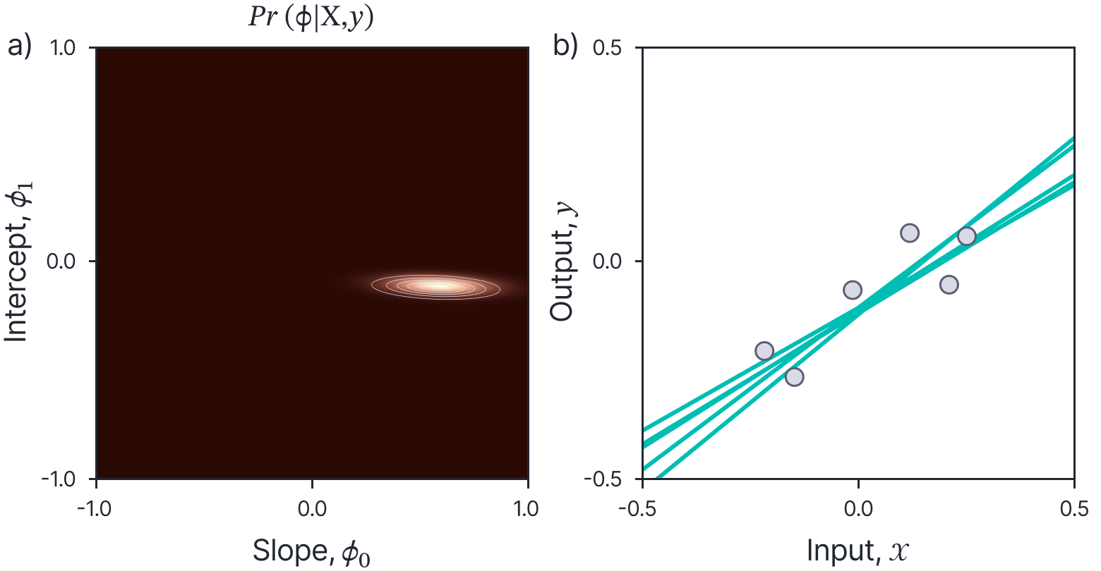
Figure 5. Posterior distribution over parameters. a) The posterior distribution $\operatorname{Pr}(\boldsymbol{\phi} \mid \mathbf{X}, \mathbf{y})$ reflects what we know about the parameters after we have observed that training data $\mathbf{X}, \mathbf{y}$. This is naturally more concentrated than the prior distribution. b) Samples from the posterior distribution. Each corresponds to a different line that plausibly passes through the data.
We now compute the predictive distribution over the prediction $y^{*}$ for a new data vector $\mathbf{x}^{*}$.
\begin{equation*}
\operatorname{Pr}\left(y^{*} \mid \mathbf{x}^{*}, \mathbf{X}, \mathbf{y}\right)=\int \operatorname{Pr}\left(y^{*} \mid \mathbf{x}^{*}, \boldsymbol{\phi}\right) \operatorname{Pr}(\boldsymbol{\phi} \mid \mathbf{X}, \mathbf{y}) d \boldsymbol{\phi}, \tag{18}
\end{equation*}
where the first term on the right-hand side is given by:
\begin{equation*}
\operatorname{Pr}\left(y^{*} \mid \mathbf{x}^{*}, \boldsymbol{\phi}\right)=\operatorname{Norm}_{y^{*}}\left[\boldsymbol{\phi}^{T} \mathbf{x}^{*}, \sigma_{n}^{2}\right], \tag{19}
\end{equation*}
and the second term by equation 17.
The integral can be performed by applying the first relations in equations 1.16 which yield a normal distribution in $\boldsymbol\phi$ which integrates to one, leaving behind the constant $\kappa_{1}$, which itself is a normal distribution in $y^{*}$ (see proof at end of blog):
\begin{align*}
& \operatorname{Pr}\left(y^{*} \mid \mathbf{x}^{*}, \mathbf{X}, \mathbf{y}\right)= \tag{20}\\
&\hspace{1cm} \operatorname{Norm}_{y^{*}}\left[\mathbf{x}^{* T}\left(\mathbf{X} \mathbf{X}^{T}+\frac{\sigma_{n}^{2}}{\sigma_{p}^{2}} \mathbf{I}\right)^{-1} \mathbf{X} \mathbf{y}, \sigma_{n}^{2} \mathbf{x}^{* T}\left(\mathbf{X X}^{T}+\frac{\sigma_{n}^{2}}{\sigma_{p}^{2}} \mathbf{I}\right)^{-1} \mathbf{x}^{*}+\sigma_{n}^{2}\right].
\end{align*}
This Bayesian formulation of linear regression (figure 6) is less confident about its predictions, and the confidence decreases as the test data $\mathbf{x}^{*}$ departs from the mean $\overline{\mathbf{x}}$ of the observed data. This is because uncertainty in the gradient causes increasing uncertainty in the predictions as we move further away from the bulk of the data. This agrees with our intuitions: predictions ought to become less confident as we extrapolate further from the data.

Figure 6. Predictive distribution Bayesian linear regression. a) Predictive distribution without added noise term (i.e., without the last term in the variance in equation 1.20). Cyan line represents the mean of the distribution. Shaded area shows $\pm 2$ standard deviations. This distribution shows where we expect the true function to lie. b) Predictive distribution with added noise term. This shows where we expect the data to lie.
Practical concerns
To implement this model we must compute the $D \times D$ matrix inverse terms in equation 20. If the dimension $D$ of the original data is large then it will be difficult to compute this inverse directly.
Fortunately, this term can be inverted far more efficiently when the number of data points $I$ is fewer than the number of dimensions $D$. We use the following two matrix inversion identities (see proofs at end of blog):
\begin{align*}
\left(\mathbf{A}^{-1}+\mathbf{B}^{T} \mathbf{C}^{-1} \mathbf{B}\right)^{-1} \mathbf{B}^{T} \mathbf{C}^{-1} & =\mathbf{A} \mathbf{B}^{T}\left(\mathbf{B A} \mathbf{B}^{T}+\mathbf{C}\right)^{-1} \\
\left(\mathbf{A}^{-1}+\mathbf{B}^{T} \mathbf{C}^{-1} \mathbf{B}\right)^{-1} & =\mathbf{A}-\mathbf{A} \mathbf{B}^{T}\left(\mathbf{B A} \mathbf{B}^{T}+\mathbf{C}\right)^{-1} \mathbf{B A}, \tag{21}
\end{align*}
which are valid when $\mathbf{A}$ and $\mathbf{C}$ are symmetric and positive definite. Applying the first identity to the inverse component in the mean of 20, and the second identity to the inverse component in the variance, we respectively yield:
\begin{align*}
\mathbf{x}^{* T}\left(\mathbf{X X}^{T}+\frac{\sigma_{n}^{2}}{\sigma_{p}^{2}} \mathbf{I}_{D}\right)^{-1} \mathbf{X} & =\mathbf{x}^{* T} \mathbf{X}\left(\mathbf{X}^{T} \mathbf{X}+\frac{\sigma_{p}^{2}}{\sigma_{n}^{2}} \mathbf{I}_{I}\right)^{-1} \tag{22}\\
\left(\mathbf{X} \mathbf{X}^{T}+\frac{\sigma_{n}^{2}}{\sigma_{p}^{2}} \mathbf{I}_{D}\right)^{-1} & =\frac{\sigma_{p}^{2}}{\sigma_{n}^{2}} \mathbf{I}_{D}-\frac{\sigma_{p}^{2}}{\sigma_{n}^{2}} \mathbf{X}\left(\mathbf{X}^{T} \mathbf{X}+\frac{\sigma_{n}^{2}}{\sigma_{p}^{2}} \mathbf{I}_{I}\right)^{-1} \mathbf{X}^{T},
\end{align*}
where we have explicitly noted the dimensionality of each of the identity matrices $\mathbf{I}$ as a subscript. This expression still includes inversions but now they are of size $I \times I$ where $I$ is the number of examples: if the number of data examples $I$ is less than the data dimensionality $D$ then this formulation is more practical.
Substituting these two inversion results back into equation 20, we get a new formula for the predictive distribution:
\begin{align*}
\operatorname{Pr}\left(y^{*} \mid \mathbf{x}^{*}, \mathbf{X}, \mathbf{y}\right)=\operatorname{Norm}_{y^{*}}\Biggl[ & \mathbf{x}^{* T} \mathbf{X}\biggl(\mathbf{X}^{T} \mathbf{X}+\frac{\sigma_{n}^{2}}{\sigma_{p}^{2}} \mathbf{I}\biggr)^{-1} \mathbf{y}, \tag{23}\\
& \sigma_{p}^{2} \mathbf{x}^{* T} \mathbf{x}^{*}-\sigma_{p}^{2} \mathbf{x}^{* T} \mathbf{X}\biggl(\mathbf{X}^{T} \mathbf{X}+\frac{\sigma^{2}}{\sigma_{p}^{2}} \mathbf{I}\biggr)^{-1} \mathbf{X}^{T} \mathbf{x}^{*}+\sigma_{n}^{2}\Biggr].
\end{align*}
It is notable that only inner products of the data vectors (e.g., in the terms $\mathbf{X}^T \mathbf{x}^{*}$, or $\mathbf{X} \mathbf{X}^{T}$ ) are required to compute this expression. We will exploit this fact when we generalize these ideas to non-linear regression (see the next article part V of this series of blogs).
Conclusion
This blog has discussed the Bayesian approach to machine learning from a parameter viewpoint. Instead of choosing a single set of ‘best’ parameters, we acknowledge that there are many choices that are compatible with the data. To make predictions we take an infinite weighted sum of all possible parameter choices, where the weight depends on the compatibility. We work through the example of linear regression, for which a closed form solution is available.
These ideas can be easily extended to classification tasks (see Prince, 2012) and to certain types of non-linear model (see part V of this series). However, as we shall see in subsequent articles, they struggle with more complex models such as neural networks.
The next article in this series (part V) also discusses the Bayesian viewpoint, but this time considers it from the Gaussian processes viewpoint which focuses on the output function. We define a prior directly on the output function which defines a joint distribution between data points. We perform inference by finding the conditional distribution of the function at unknown points give the observed values of the function at the known points. For the linear regression model, this yields exactly the same predictive distribution as the methods in this blog. However, as we shall see in future articles, it has quite different implications for more complex models like deep neural networks.
Change of variables relation
The change of variables relation (figure 7) for multivariate normals states that:
\begin{equation}\operatorname{Norm}_{\mathbf{x}}[\mathbf{A y}+\mathbf{b}, \boldsymbol{\Sigma}]=\kappa_{1} \cdot \operatorname{Norm}_{\mathbf{y}}\left[\left(\mathbf{A}^{T} \boldsymbol{\Sigma}^{-1} \mathbf{A}\right)^{-1} \mathbf{A}^{T} \boldsymbol{\Sigma}^{-1}(\mathbf{x}-\mathbf{b}),\left(\mathbf{A}^{T} \boldsymbol{\Sigma}^{-1} \mathbf{A}\right)^{-1}\right].
\end{equation}
Proof:
\begin{aligned}
\operatorname{Norm}_{\mathbf{x}}[\mathbf{A y}+\mathbf{b}, \boldsymbol{\Sigma}] & =\kappa_{1} \exp \left[-0.5\left((\mathbf{x}-\mathbf{b}-\mathbf{A} \mathbf{y})^{T} \boldsymbol{\Sigma}^{-1}(\mathbf{x}-\mathbf{b}-\mathbf{A} \mathbf{y})\right)\right] \\
& =\kappa_{2} \exp \left[-0.5\left(\mathbf{y}^{T} \mathbf{A}^{T} \boldsymbol{\Sigma}^{-1} \mathbf{A} \mathbf{y}-2 \mathbf{y}^{T} \mathbf{A}^{T} \boldsymbol{\Sigma}^{-1}(\mathbf{x}-\mathbf{b})\right)\right],
\end{aligned}
where we have expanded the quadratic term and absorbed the term that does not depend on $\mathbf{y}$ into a new constant $\kappa_{3}$. Now we complete the square to make a new distribution in the variable $\mathbf{y}$:
\begin{aligned}
& \operatorname{Norm}_{\mathbf{x}}[\mathbf{A y}+\mathbf{b}, \mathbf{\Sigma}] \\
& \hspace{2cm}=\kappa_{2} \exp \left[-0.5\left(\mathbf{y}^{T} \mathbf{A}^{T} \boldsymbol{\Sigma}^{-1} \mathbf{A} \mathbf{y}-2 \mathbf{y}^{T} \mathbf{A}^{T} \boldsymbol{\Sigma}^{-1}(\mathbf{x}-\mathbf{b})\right)\right] \\
& \hspace{2cm}=\kappa_{3} \exp \left[-0.5\left(\mathbf{y}^{T} \mathbf{A}^{T} \boldsymbol{\Sigma}^{-1} \mathbf{A} \mathbf{y}-2 \mathbf{y}^{T} \mathbf{A}^{T} \boldsymbol{\Sigma}^{-1}(\mathbf{x}-\mathbf{b})\right.\right. \\
& \hspace{4cm}\left.\left.-2(\mathbf{x}-\mathbf{b})^{T} \boldsymbol{\Sigma}^{-1} \mathbf{A}^{T}\left(\mathbf{A}^{T} \boldsymbol{\Sigma}^{-1} \mathbf{A}\right)^{-1} \mathbf{A} \boldsymbol{\Sigma}^{-1}(\mathbf{x}-\mathbf{b})\right)\right] \\
& \hspace{2cm}=\kappa_{3} \exp \left[-0.5\left(\left(\mathbf{y}-\left(\mathbf{A}^{T} \boldsymbol{\Sigma}^{-1} \mathbf{A}\right)^{-1} \mathbf{A} \boldsymbol{\Sigma}^{-1}(\mathbf{x}-\mathbf{b})\right)^{T}\left(\mathbf{A}^{T} \boldsymbol{\Sigma}^{-1} \mathbf{A}\right)\right.\right. \\
& \hspace{4cm}\left.\left.\left(\mathbf{y}-\left(\mathbf{A}^{T} \boldsymbol{\Sigma}^{-1} \mathbf{A}\right)^{-1} \mathbf{A} \boldsymbol{\Sigma}^{-1}(\mathbf{x}-\mathbf{b})\right)\right)\right] \\
& \hspace{2cm}=\kappa_{4} \operatorname{Norm}_{\mathbf{y}}\left[\left(\mathbf{A}^{T} \boldsymbol{\Sigma}^{-1} \mathbf{A}\right)^{-1} \mathbf{A} \boldsymbol{\Sigma}^{-1}(\mathbf{x}-\mathbf{b}),\left(\mathbf{A}^{T} \boldsymbol{\Sigma}^{-1} \mathbf{A}\right)^{-1}\right],
\end{aligned}
as required.
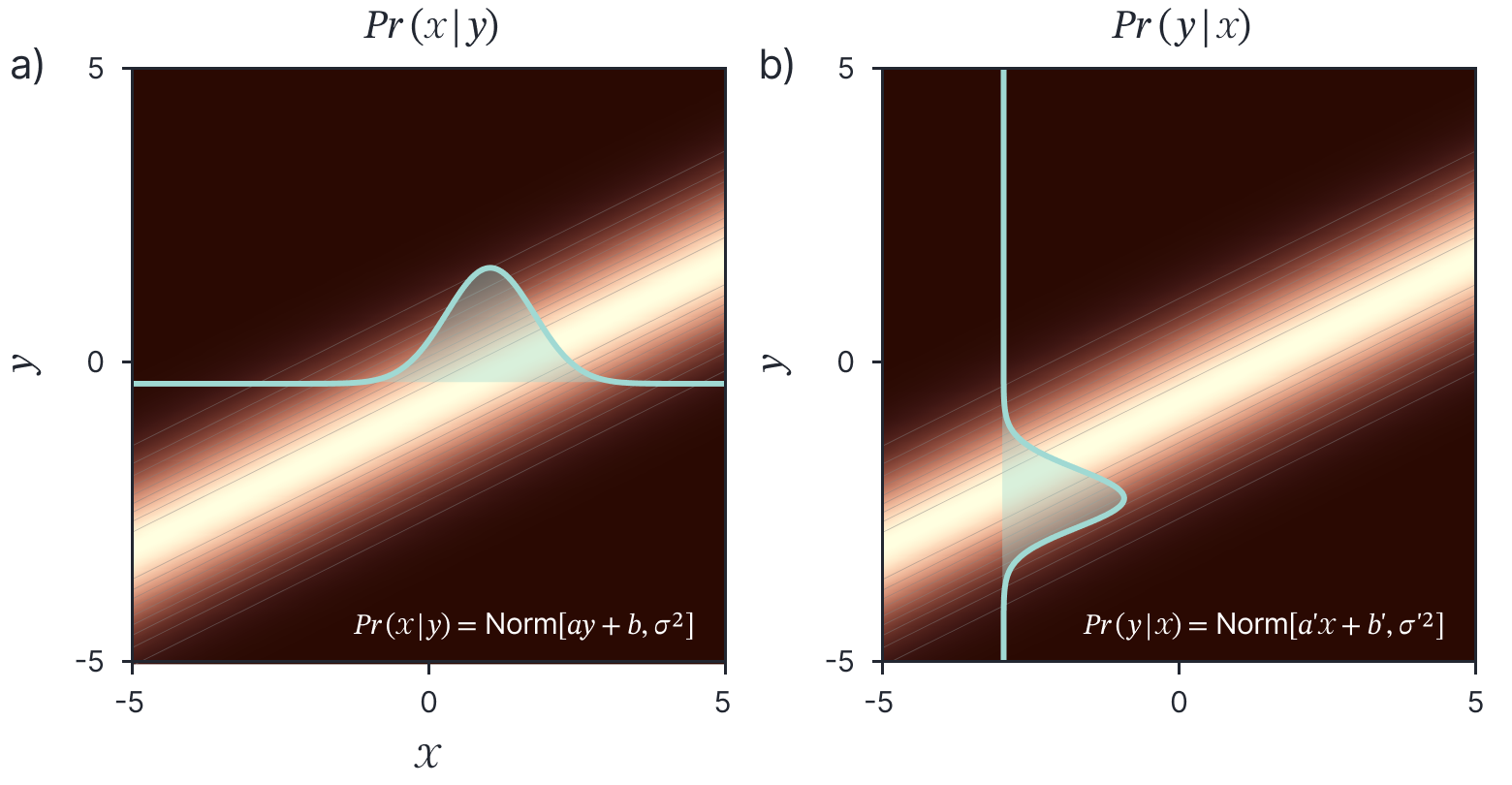
Figure 7. Change of variables relation. A normal distribution in $x$ that has a mean that is a linear function of a second variable $y$ is proportional to a normal distribution in y with a mean that is a linear function of $x$.
Product of two Gaussians
The product of two Gaussians is another Gaussian:
\begin{aligned}
\operatorname{Norm}_{\mathbf{x}}[\mathbf{a}, \mathbf{A}] \operatorname{Norm}_{\mathbf{x}}[\mathbf{b}, \mathbf{B}] \propto \operatorname{Norm}_{\mathbf{x}}\left[\left(\mathbf{A}^{-1}+\mathbf{B}^{-1}\right)^{-1}\left(\mathbf{A}^{-1} \mathbf{a}+\mathbf{B}^{-1} \mathbf{b}\right),\left(\mathbf{A}^{-1}+\mathbf{B}^{-1}\right)^{-1}\right].
\end{aligned}
Proof: We first write out the expression for the product of the normals:
\begin{aligned}
\mbox{Norm}_\mathbf{x}\left[\mathbf{a},\mathbf{A}\right]\mbox{Norm}_{\mathbf{x}}\left[\mathbf{b},\mathbf{B}\right]&\\
&\hspace{-2cm}=\kappa_{1} \exp \left[-0.5(\mathbf{x}-\mathbf{a})^{T} \mathbf{A}^{-1}(\mathbf{x}-\mathbf{a})-0.5(\mathbf{x}-\mathbf{b})^{T} \mathbf{B}^{-1}(\mathbf{x}-\mathbf{b})\right] \\
& \hspace{-2cm}=\kappa_{2} \exp \left[-0.5\left(\mathbf{x}^{T}\left(\mathbf{A}^{-1}+\mathbf{B}^{-1}\right) \mathbf{x}+2\left(\mathbf{A}^{-1} \mathbf{a}+\mathbf{B}^{-1} \mathbf{b}\right) \mathbf{x}\right)\right],
\end{aligned}
where we have multiplied out the terms in the exponential and subsumed the terms that are constant in $\mathbf{x}$ into a new constant $\kappa_{2}$.
Now we complete the square by multiplying and dividing by a new term, creating a new constant $\kappa_{3}$ :
\begin{aligned}
\mbox{Norm}_\mathbf{x}\left[\mathbf{a},\mathbf{A}\right]\mbox{Norm}_{\mathbf{x}}\left[\mathbf{b},\mathbf{B}\right]&\\
& \hspace{-2cm}=\kappa_{2} \exp \left[-0.5\left(\mathbf{x}^{T}\left(\mathbf{A}^{-1}+\mathbf{B}^{-1}\right) \mathbf{x}+2\left(\mathbf{A}^{-1} \mathbf{a}+\mathbf{B}^{-1} \mathbf{b}\right) \mathbf{x}\right)\right] \\
& \hspace{-2cm}=\kappa_{3} \exp \left[-0.5\left(\mathbf{x}^{T}\left(\mathbf{A}^{-1}+\mathbf{B}^{-1}\right) \mathbf{x}+2\left(\mathbf{A}^{-1} \mathbf{a}+\mathbf{B}^{-1} \mathbf{b}\right) \mathbf{x}\right.\right. \\
& \left.\left.+\left(\mathbf{A}^{-1} \mathbf{a}+\mathbf{B}^{-1} \mathbf{b}\right)^{T}\left(\mathbf{A}^{-1}+\mathbf{B}^{-1}\right)^{-1}\left(\mathbf{A}^{-1} \mathbf{a}+\mathbf{B}^{-1} \mathbf{b}\right)\right)\right].
\end{aligned}
Finally, we re-factor the exponential term into the form of a standard normal distribution, and divide and multiply by the associated constant term for this new normal distribution, creating a new constant $\kappa_{4}$ :
\begin{aligned}
\mbox{Norm}_\mathbf{x}\left[\mathbf{a},\mathbf{A}\right]\mbox{Norm}_{\mathbf{x}}\left[\mathbf{b},\mathbf{B}\right]&\\
&\hspace{-2cm} = \kappa_{3} \exp \left[-0.5\left(\mathbf{x}-\left(\mathbf{A}^{-1}+\mathbf{B}^{-1}\right)^{-1}\left(\mathbf{A}^{-1} \mathbf{a}+\mathbf{B}^{-1} \mathbf{b}\right)\right)^{T}\left(\mathbf{A}^{-1}+\mathbf{B}^{-1}\right)\right. \\
& \hspace{2cm}\left.\left(\mathbf{x}-\left(\mathbf{A}^{-1}+\mathbf{B}^{-1}\right)^{-1}\left(\mathbf{A}^{-1} \mathbf{a}+\mathbf{B}^{-1} \mathbf{b}\right)\right)\right] \\
& \hspace{-2cm}= \kappa_{4} \operatorname{Norm}_{\mathbf{x}}\left[\left(\mathbf{A}^{-1}+\mathbf{B}^{-1}\right)^{-1}\left(\mathbf{A}^{-1} \mathbf{a}+\mathbf{B}^{-1} \mathbf{b}\right),\left(\mathbf{A}^{-1}+\mathbf{B}^{-1}\right)^{-1}\right].
\end{aligned}
Constant of proportionality
The constant of proportionality $\kappa$ in the above product relation is also a normal distribution where:
$$
\kappa=\operatorname{Norm}_{\mathbf{a}}[\mathbf{b}, \mathbf{A}+\mathbf{B}].
$$
Proof: We will compute each of the constants in the previous section in turn.
$$
\begin{aligned}
\kappa_{1} & =\frac{1}{(2 \pi)^{D}|\mathbf{A}|^{0.5}|\mathbf{B}|^{0.5}} \\
\kappa_{2} & =\kappa_{1} \cdot \exp \left[-0.5 \mathbf{a}^{T} \mathbf{A}^{-1} \mathbf{a}-0.5 \mathbf{b}^{T} \mathbf{B}^{-1} \mathbf{b}\right] \\
\kappa_{3} & =\kappa_{2} \cdot \exp \left[0.5\left(\mathbf{A}^{-1} \mathbf{a}+\mathbf{B}^{-1} \mathbf{b}\right)^{T}\left(\mathbf{A}^{-1}+\mathbf{B}^{-1}\right)^{-1}\left(\mathbf{A}^{-1} \mathbf{a}+\mathbf{B}^{-1} \mathbf{b}\right)\right] \\
\kappa_{4} & =\kappa_{3} \cdot 2 \pi^{D / 2}\left|\left(\mathbf{A}^{-1}+\mathbf{B}^{-1}\right)^{-1}\right|^{0.5}
\end{aligned}.
$$
Working first with the non-exponential terms, we have
\begin{aligned}
\kappa & =\frac{1}{(2 \pi)^{D}|\mathbf{A}|^{0.5}|\mathbf{B}|^{0.5}} \cdot 2 \pi^{D / 2}\left|\left(\mathbf{A}^{-1}+\mathbf{B}^{-1}\right)^{-1}\right|^{0.5} \exp [\bullet] \\
& =\frac{1}{2 \pi^{D / 2}|\mathbf{A}|^{0.5}|| \mathbf{A}^{-1}+\left.\mathbf{B}^{-1}\right|^{0.5}|\mathbf{B}|^{0.5}} \exp [\bullet] \\
& =\frac{1}{2 \pi^{D / 2}|\mathbf{A}+\mathbf{B}|^{0.5}} \exp [\bullet],
\end{aligned}
which is the appropriate constant for the normal distribution. Returning to the exponential term, we have:
\begin{aligned}
\kappa & \propto \exp \left[-0.5\left(\mathbf{a}^{T} \mathbf{A}^{-1} \mathbf{a}+\mathbf{b}^{T} \mathbf{B}^{-1} \mathbf{b}\right.\right. \\
&\hspace{2cm}\left.\left.-\left(\mathbf{A}^{-1} \mathbf{a}+\mathbf{B}^{-1} \mathbf{b}\right)^{T}\left(\mathbf{A}^{-1}+\mathbf{B}^{-1}\right)^{-1}\left(\mathbf{A}^{-1} \mathbf{a}+\mathbf{B}^{-1} \mathbf{b}\right)\right)\right] \\
& \propto \exp \left[-0.5\left(\mathbf{a}^{T} \mathbf{A}^{-1} \mathbf{a}+\mathbf{b}^{T} \mathbf{B}^{-1} \mathbf{b}-\mathbf{a}^{T} \mathbf{A}^{-1}\left(\mathbf{A}^{-1}+\mathbf{B}^{-1}\right)^{-1} \mathbf{A}^{-1} \mathbf{a}\right.\right. \\
&\hspace{2cm}\left.\left.-\mathbf{b}^{T} \mathbf{B}^{-1}\left(\mathbf{A}^{-1}+\mathbf{B}^{-1}\right)^{-1} \mathbf{B}^{-1} \mathbf{b}-2 \mathbf{a}^{T} \mathbf{A}^{-1}\left(\mathbf{A}^{-1}+\mathbf{B}^{-1}\right)^{-1} \mathbf{B}^{-1} \mathbf{b}\right)\right] \\
& \propto \exp \left[-0.5\left(\mathbf{a}^{T} \mathbf{A}^{-1} \mathbf{a}+\mathbf{b}^{T} \mathbf{B}^{-1} \mathbf{b}-\mathbf{a}^{T} \mathbf{A}^{-1}\left(\mathbf{A}^{-1}+\mathbf{B}^{-1}\right)^{-1} \mathbf{A}^{-1} \mathbf{a}\right.\right. \\
&\hspace{2cm}\left.\left.-\mathbf{b}^{T} \mathbf{B}^{-1}\left(\mathbf{A}^{-1}+\mathbf{B}^{-1}\right)^{-1} \mathbf{B}^{-1} \mathbf{b}-2 \mathbf{a}^{T}(\mathbf{A}+\mathbf{B})^{-1} \mathbf{b}\right)\right] \\
& \propto \exp \left[-0.5\left(\mathbf{a}^{T} \mathbf{A}^{-1} \mathbf{a}+\mathbf{b}^{T} \mathbf{B}^{-1} \mathbf{b}-\mathbf{a}^{T}(\mathbf{A}+\mathbf{B})^{-1} \mathbf{B} \mathbf{A}^{-1} \mathbf{a}\right.\right. \\
&\hspace{2cm}\left.\left.-\mathbf{b}^{T}(\mathbf{A}+\mathbf{B})^{-1} \mathbf{A} \mathbf{B}^{-1} \mathbf{b}-2 \mathbf{a}^{T}(\mathbf{A}+\mathbf{B})^{-1} \mathbf{b}\right)\right].
\end{aligned}
Now we use the identities
\begin{aligned}
\mathbf{a}^{T} \mathbf{A}^{-1} \mathbf{a} & =\mathbf{a}^{T}(\mathbf{A}+\mathbf{B})^{-1}(\mathbf{A}+\mathbf{B}) \mathbf{A}^{-1} \mathbf{a} \\
& =\mathbf{a}^{T}(\mathbf{A}+\mathbf{B})^{-1} \mathbf{a}+\mathbf{a}^{T}(\mathbf{A}+\mathbf{B})^{-1} \mathbf{B} \mathbf{A}^{-1} \mathbf{a}
\end{aligned}
and
\begin{aligned}
\mathbf{b}^{T} \mathbf{B}^{-1} \mathbf{b} & =\mathbf{b}^{T}(\mathbf{A}+\mathbf{B})^{-1}(\mathbf{A}+\mathbf{B}) \mathbf{B}^{-1} \mathbf{b} \\
& =\mathbf{b}^{T}(\mathbf{A}+\mathbf{B})^{-1} \mathbf{b}+\mathbf{b}^{T}(\mathbf{A}+\mathbf{B})^{-1} \mathbf{A} \mathbf{B}^{-1} \mathbf{b}.
\end{aligned}
Substituting these into the main equation we get:
\begin{aligned}
\kappa & \propto \exp \left[-0.5\left(\mathbf{a}^{T} \mathbf{A}^{-1} \mathbf{a}+\mathbf{b}^{T} \mathbf{B}^{-1} \mathbf{b}-\mathbf{a}^{T}(\mathbf{A}+\mathbf{B})^{-1} \mathbf{B} \mathbf{A}^{-1} \mathbf{a}\right.\right. \\
& \hspace{3cm}\left.\left.-\mathbf{b}^{T}(\mathbf{A}+\mathbf{B})^{-1} \mathbf{A} \mathbf{B}^{-1} \mathbf{b}-2 \mathbf{a}^{T}(\mathbf{A}+\mathbf{B})^{-1} \mathbf{b}\right)\right] \\
& \propto \exp \left[-0.5\left(\mathbf{a}^{T}(\mathbf{A}+\mathbf{B})^{-1} \mathbf{a}+\mathbf{b}^{T}(\mathbf{A}+\mathbf{B})^{-1} \mathbf{b}-2 \mathbf{a}^{T}(\mathbf{A}+\mathbf{B})^{-1} \mathbf{b}\right)\right] \\
& \propto \exp \left[-0.5(\mathbf{a}-\mathbf{b})^{T}(\mathbf{A}+\mathbf{B})^{-1}(\mathbf{a}-\mathbf{b})\right].
\end{aligned}
Putting this together with the constant term we have:
$$
\kappa=\operatorname{Norm}_{\mathbf{a}}[\mathbf{b}, \mathbf{A}+\mathbf{B}],
$$
as required.
Inversion relation #1
Consider the $d \times d$ matrix $\mathbf{A}$, the $k \times k$ matrix $\mathbf{C}$ and the $k \times d$ matrix $\mathbf{B}$ where $\mathbf{A}$ and $\mathbf{C}$ are symmetric, positive definite covariance matrices. The following equality holds:
\begin{equation*}
\left(\mathbf{A}^{-1}+\mathbf{B}^{T} \mathbf{C}^{-1} \mathbf{B}\right)^{-1} \mathbf{B}^{T} \mathbf{C}^{-1}=\mathbf{A} \mathbf{B}^{T}\left(\mathbf{B A} \mathbf{B}^{T}+\mathbf{C}\right)^{-1} .\tag{25}
\end{equation*}
Proof:
\begin{align*}
\mathbf{B}^{T}+\mathbf{B}^{T} \mathbf{C}^{-1} \mathbf{B} \mathbf{A} \mathbf{B}^{T} & =\mathbf{B}^{T} \mathbf{C}^{-1} \mathbf{B} \mathbf{A} \mathbf{B}^{T}+\mathbf{B}^{T} \\
\left(\mathbf{A}^{-1}+\mathbf{B}^{T} \mathbf{C}^{-1} \mathbf{B}\right) \mathbf{A} \mathbf{B}^{T} & =\mathbf{B}^{T} \mathbf{C}^{-1}\left(\mathbf{B A} \mathbf{B}^{T}+\mathbf{C}\right).
\end{align*}
Premultiplying the both sides by $\left(\mathbf{A}^{-1}+\mathbf{B}^{T} \mathbf{C}^{-1} \mathbf{B}\right)^{-1}$ and post-multplying by $\left(\mathbf{B A B}{ }^{T}+\right.$ $\mathbf{C})^{-1}$, we get:
\begin{equation*}
\left(\mathbf{A}^{-1}+\mathbf{B}^{T} \mathbf{C}^{-1} \mathbf{B}\right)^{-1} \mathbf{B}^{T} \mathbf{C}^{-1}=\mathbf{A} \mathbf{B}^{T}\left(\mathbf{B A} \mathbf{B}^{T}+\mathbf{C}\right)^{-1}, \tag{27}
\end{equation*}
as required.
Inversion relation #2: Sherman-Morrison-Woodbury
Consider the $d \times d$ matrix $\mathbf{A}$, the $k \times k$ matrix $\mathbf{C}$ and the $k \times d$ matrix $\mathbf{B}$ where $\mathbf{A}$ and $\mathbf{C}$ are symmetric, positive definite covariance matrices. The following equality holds:
\begin{equation*}
\left(\mathbf{A}^{-1}+\mathbf{B}^{T} \mathbf{C}^{-1} \mathbf{B}\right)^{-1}=\mathbf{A}-\mathbf{A} \mathbf{B}^{T}\left(\mathbf{B A} \mathbf{B}^{T}+\mathbf{C}\right)^{-1} \mathbf{B} \mathbf{A}. \tag{28}
\end{equation*}
This is sometimes known as the matrix inversion lemma.
Proof:
\begin{align*}
\left(\mathbf{A}^{-1}+\mathbf{B}^{T}\right. & \left.\mathbf{C}^{-1} \mathbf{B}\right)^{-1} \\
& =\left(\mathbf{A}^{-1}+\mathbf{B}^{T} \mathbf{C}^{-1} \mathbf{B}\right)^{-1}\left(\mathbf{I}+\mathbf{B}^{T} \mathbf{C}^{-1} \mathbf{B} \mathbf{A}-\mathbf{B}^{T} \mathbf{C}^{-1} \mathbf{B A}\right) \\
& =\left(\mathbf{A}^{-1}+\mathbf{B}^{T} \mathbf{C}^{-\mathbf{1}} \mathbf{B}\right)^{-1}\left(\left(\mathbf{A}^{-1}+\mathbf{B}^{T} \mathbf{C}^{-1} \mathbf{B}\right) \mathbf{A}-\mathbf{B}^{T} \mathbf{C}^{-1} \mathbf{B A}\right) \\
& =\mathbf{A}-\left(\mathbf{A}^{-1}+\mathbf{B}^{T} \mathbf{C}^{-1} \mathbf{B}\right)^{-1} \mathbf{B}^{T} \mathbf{C}^{-1} \mathbf{B} \mathbf{A}. \tag{29}
\end{align*}
Now, applying inversion relation #1 to the term in brackets:
\begin{align*}
\left(\mathbf{A}^{-1}+\mathbf{B}^{T} \mathbf{C}^{-1} \mathbf{B}\right)^{-1} & =\mathbf{A}-\left(\mathbf{A}^{-1}+\mathbf{B}^{T} \mathbf{C}^{-1} \mathbf{B}\right)^{-1} \mathbf{B} \mathbf{C}^{-1} \mathbf{B A} \\
& =\mathbf{A}-\mathbf{A} \mathbf{B}^{T}\left(\mathbf{B} \mathbf{A} \mathbf{B}^{T}+\mathbf{C}\right)^{-1} \mathbf{B A}, \tag{30}
\end{align*}
as required.
Join our Research team
RBC Borealis is looking to hire for various roles! Visit our career page and discover opportunities to work on cutting-edge models and products positively impacting millions of Canadians.
Careers at RBC Borealis