
In part IV and part V of this series, we introduced the Bayesian approach to machine learning from the parameter space and function space perspectives, respectively. In part VI (this blog) and part VII we apply these ideas to neural networks, yielding Bayesian neural networks and neural network Gaussian processes, respectively.
For linear models, the parameter space and function space perspectives generated identical results. However, we shall see that this is not necessarily the case for non-linear models. Indeed, for deep neural networks, the function space perspective is tractable, but the parameter space perspective is not; it’s not even possible to write a closed-form expression for the posterior distribution over the parameters.
To make progress, we must make one of two kinds of approximation. We can either (i) approximate the posterior distribution as a collection of samples or (ii) approximate it with a more practical family of distributions (the variational approach). The former approach has close connections to other techniques like ensembling. We start by briefly reviewing Bayesian learning from the parameter space perspective. If you read part IV of this series of blogs, you can skip this section.
Bayesian Parameter space review
Consider a model $y=\mbox{f}[\mathbf{x},\boldsymbol\phi]$ which takes a multivariate input $\mathbf{x}$, returns a single scalar output $y$, and has parameters $\boldsymbol\phi$. We assume that we are given a training dataset $\{\mathbf{x}_{i},y_i\}_{i=1}^I$ containing $I$ input/output pairs, and that we have a noise model $Pr(y_{i}|\mathbf{x}_{i},\boldsymbol\phi)$ which specifies how likely we are to observe the training output $y_{i}$ given input $\mathbf{x}_{i}$ and model parameters $\boldsymbol\phi$. For a regression problem, this would typically be a normal distribution where the mean is specified by the model output, and the noise variance $\sigma^2_n$ is constant:
\begin{equation}
Pr(y_{i}|\mathbf{x}_{i},\boldsymbol\phi) = \mbox{Norm}_{y_{i}}\Bigl[\mbox{f}[\mathbf{x}_i,\boldsymbol\phi],\sigma^2_n\Bigr].
\tag{1}
\end{equation}
We incorporate prior information about the parameters $\boldsymbol\phi$ by defining a prior probability distribution $Pr(\boldsymbol\phi)$.
In the Bayesian approach, we apply Bayes’ rule to find a distribution over the parameters:
\begin{equation}\label{eq:Bayes3_Bayes}
Pr(\boldsymbol\phi | \{\mathbf{x}_{i},\mathbf{y}_{i}\}) = \frac{\prod_{i=1}^{I} Pr(y_{i}|\mathbf{x}_{i},\boldsymbol\phi)Pr(\boldsymbol\phi)}{\int \prod_{i=1}^{I} Pr(y_{i}|\mathbf{x}_{i},\boldsymbol\phi)Pr(\boldsymbol\phi)d\boldsymbol\phi}.
\tag{2}
\end{equation}
The left-hand side is referred to as the posterior probability of the parameters, which takes into account both the likelihood $\prod_i Pr(y_{i}|\mathbf{x}_{i},\boldsymbol\phi)$ of the parameters given the observed data, and the prior information about the parameters $Pr(\boldsymbol\phi)$. The posterior probability will be high for values that are both compatible with the data and have a high prior probability.
To perform inference (compute the estimate $y^*$ for a new input $\mathbf{x}^*$) we marginalize over (integrate over) the uncertain parameters $\boldsymbol\phi$:
\begin{equation}
Pr\bigl(y^*|\mathbf{x}^*,\{\mathbf{x}_{i},\mathbf{y}_{i}\}\bigr) = \int Pr\bigl(y^*|\mathbf{x}^*,\boldsymbol\phi\bigr) Pr\bigl(\boldsymbol\phi|\{\mathbf{x}_{i},\mathbf{y}_{i}\}\bigr) d\boldsymbol\phi.
\tag{3}
\end{equation}
This can be interpreted as weighting together the predictions of an infinitely large ensemble of models (via the integral), where there is one model $Pr\bigl(y^*|\mathbf{x}^*,\boldsymbol\phi\bigr)$ for each choice of parameters $\boldsymbol\phi.$ The weight for that model is given by the associated posterior probability $Pr\bigl(\boldsymbol\phi|\{\mathbf{x}_{i},\mathbf{y}_{i}\}\bigr)$ (i.e., a measure of how compatible it was with the training data).
Application to deep neural networks
Consider a deep neural network $y = \textbf{f}[\mathbf{x},\boldsymbol\phi]$ with $K$ hidden layers:
\begin{eqnarray}\label{eq:dnn_la1}
\mathbf{h}_{1} &=& \textbf{ReLU}\Bigl[\boldsymbol\beta_{0} +\boldsymbol\Omega_{0}\mathbf{x}\Bigr]\nonumber \\
\mathbf{h}_{k+1} &=& \textbf{ReLU}\Bigl[\boldsymbol\beta_{k} +\boldsymbol\Omega_{k}\mathbf{h}_{k}\Bigr]\hspace{1cm}\mbox{for } k\in 2,\ldots, K-1\nonumber \\
y &=& \beta_{K} +\boldsymbol\Omega_{K}\mathbf{h}_{K}.
\tag{4}\end{eqnarray}
where $\mathbf{h}_{k}$ is the vector of hidden units at the $k^{th}$ hidden layer and $\textbf{ReLU}[\mathbf{z}]$ applies the operation $\max[z_d,0]$ separately for each element $z_{d}\in\mathbf{z}$. The parameters $\boldsymbol\phi$ of this model comprise all of the weight matrices $\boldsymbol\Omega_{k}$ and bias vectors $\boldsymbol\beta_{k}$.
Prior distribution
Now consider defining a prior $Pr(\boldsymbol\phi)$ over the parameters. The most common choice is to define independent zero mean Gaussians over each of the weights and biases:
\begin{eqnarray}
\boldsymbol\beta_{k} &\sim& \mbox{Norm}_{\boldsymbol\beta_{k}}\Bigl[\mathbf{0},\sigma^2_{p}\mathbf{I} \Bigr]\hspace{2cm}\mbox{for } k\in 0,\ldots, K\nonumber \\
\boldsymbol\Omega_{k} &\sim& \mbox{Norm}_{\boldsymbol\Omega_{k}}\Bigl[\mathbf{0},\sigma^2_{p}\mathbf{I} \Bigr]\hspace{2cm}\mbox{for } k\in 0,\ldots, K,
\tag{5}\end{eqnarray}
where $\sigma^2_{p}$ is the prior variance of the parameters. We’ll write this as $Pr(\boldsymbol\phi)= \text{Norm}_{\boldsymbol\phi}[\mathbf{0},\sigma^2_{p}\mathbf{I}]$ for short. This prior has the advantage that the model’s Lipschitz constant (the fastest speed the output can change with respect to the input) monotonically increases with respect to $\sigma^2_p$ and so we can control the model robustness (Blaas and Roberts, 2021).
However, careful consideration reveals that this prior is rather strange. The non-negative homogeneity property of the ReLU activation function implies that for $\alpha\in\mathbb{R}^{+}$:
\begin{equation}
\mbox{ReLU}[\alpha \cdot z] = \alpha \cdot \mbox{ReLU}[z].
\tag{6}
\end{equation}
Hence, we can multiply the weights and biases that input a single layer by any positive constant and divide the output weights by the same constant and the network will produce the same result. However, the Gaussian prior implies a squared dependence on the magnitude of the parameters, so in general the prior will assign different probabilities to these equivalent models. This doesn’t pose any practical problems, but it is inelegant.
There are other choices of prior that sidestep this problem. For example, Flam-Shepherd et al. (2017) and Tran et al. (2022) learn priors whose distribution favors functions similar to some pre-specified Gaussian processes. The kernels of the Gaussian processes can be chosen manually to have desirable properties (e.g., periodicity). Similarly, Nalisnick et al., 2020 introduce predictive complexity priors that penalize discrepancies between the network and some other simpler model. Regardless, the Gaussian prior is still most commonly used.
Posterior distribution
To compute the posterior distribution, we use Bayes’ rule:
\begin{equation}\label{eq:Bayes3_Bayes2}
Pr(\boldsymbol\phi | \{\mathbf{x}_{i},\mathbf{y}_{i}\}) = \frac{\prod_{i=1}^{I} Pr(y_{i}|\mathbf{x}_{i},\boldsymbol\phi)Pr(\boldsymbol\phi)}{\int \prod_{i=1}^{I} Pr(y_{i}|\mathbf{x}_{i},\boldsymbol\phi)Pr(\boldsymbol\phi)d\boldsymbol\phi},
\tag{7}
\end{equation}
with likelihood and prior:
\begin{eqnarray}
Pr(y_{i}|\mathbf{x}_{i},\boldsymbol\phi) &=& \text{Norm}_{y_{i}}\Bigl[\textbf{f}\bigl[\mathbf{x}_{i},\boldsymbol\phi\bigr],\sigma^2_{n} \Bigr]\nonumber \\
Pr(\boldsymbol\phi)&=& \text{Norm}_{\boldsymbol\phi}\Bigl[\mathbf{0},\sigma^2_{p}\mathbf{I}\Bigr].
\tag{8}
\end{eqnarray}
Unfortunately, however, this is intractable. There is no closed-form expression for the denominator of the right-hand side of equation 7 (technically, the prior is no longer “conjugate” to the the likelihood). This means we cannot write an expression for the left-hand side either. In fact, it’s difficult to imagine that we would ever be able to do this; it takes considerable memory just to store the parameters of a modern deep network, so storing a full distribution over these parameters would be extremely challenging.
This limitation means that we cannot use the Bayesian approach without approximating the posterior distribution in some way. There are two main approaches (figure 1). In the sampling approach, we approximate the posterior distribution with a set of samples. In the variational approach we define a more tractable form for the posterior distribution and manipulate it’s parameters so that it is as close as possible to the true posterior. The next two sections consider each of these approaches in turn.
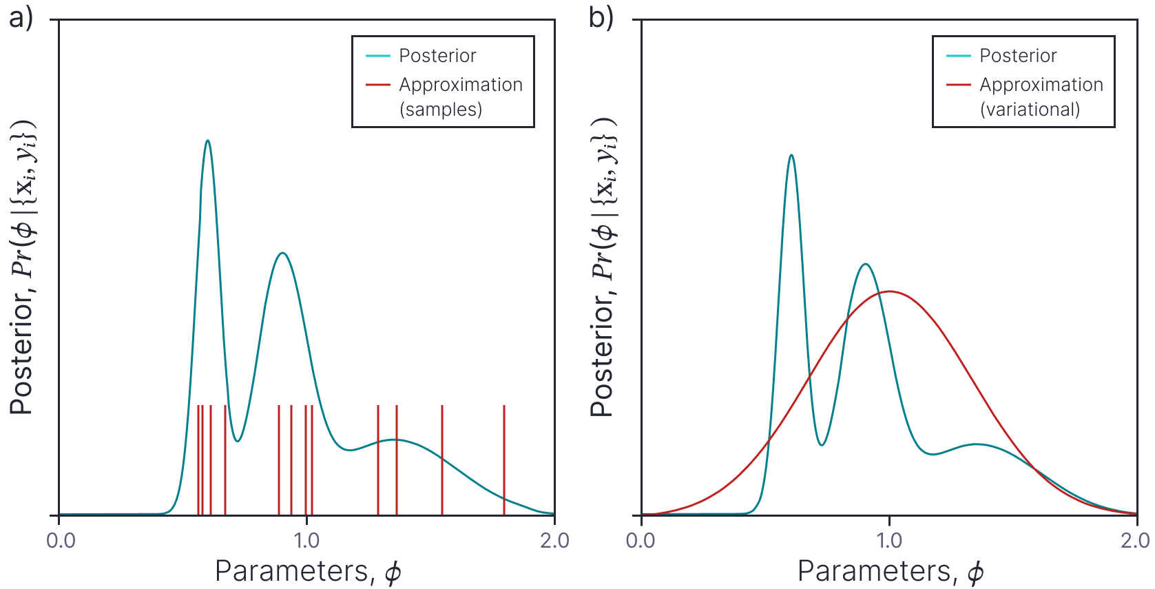
Figure 1. Posterior approximations. The posterior distribution over the parameters (cyan curve) is complex and cannot be written in closed from. We can either a) approximate this distribution with a set of samples or b) approximate it with a simpler tractable distribution (here a Gaussian).
Sampling approaches
Although we cannot compute the entire posterior distribution, we can calculate the posterior probability for a particular set of parameters $\boldsymbol\phi$ up to an unknown constant (due to the unknown denominator). This at least means we can compare the relative posterior probability of different individual parameter settings. In principle, this is sufficient to allow us to draw samples $\boldsymbol\phi^{*}_{1},\boldsymbol\phi^{*}_{2},\ldots \boldsymbol\phi^{*}_{S}$ from the posterior distribution $ Pr(\boldsymbol\phi | \{\mathbf{x}_{i},\mathbf{y}_{i}\})$. We can then approximate this distribution with the samples.
\begin{equation}
Pr(\boldsymbol\phi | \{\mathbf{x}_{i},\mathbf{y}_{i}\}) \approx \frac{1}{S}\sum_{s=1}^S\delta\bigl[\boldsymbol\phi-\boldsymbol\phi^{*}_{s}\bigr],
\tag{9}
\end{equation}
where $\delta[z]$ is a Dirac delta function which has probability mass of one at position $z$ and zero elsewhere.
It is then easy to make predictions:
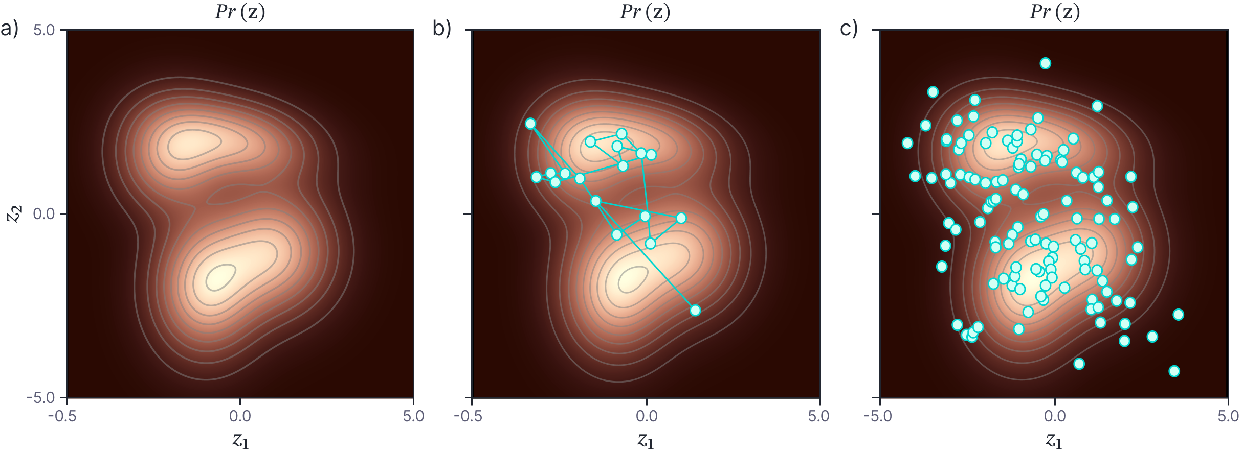
Figure 2. MCMC Sampling. a) This distribution has some complex form that does not admit a simple sampling method. b) MCMC methods generate a “chain” of samples which (after some burn-in period) represent draws from the underlying distribution. c) Points drawn from this probability distribution using the Metropolis-Hastings method.
\begin{eqnarray}\label{eq:Bayes3samplepredict}
Pr\bigl(y^*|\mathbf{x}^*,\{\mathbf{x}_{i},\mathbf{y}_{i}\}\bigr) &=& \int Pr\bigl(y^*|\mathbf{x}^*,\boldsymbol\phi\bigr) Pr\bigl(\boldsymbol\phi|\{\mathbf{x}_{i},\mathbf{y}_{i}\}\bigr) d\boldsymbol\phi\nonumber \\
&\approx & \frac{1}{S}\sum_{s=1}^S\int Pr\bigl(y^*|\mathbf{x}^*,\boldsymbol\phi\bigr) \delta\bigl[\boldsymbol\phi-\boldsymbol\phi^{*}_{s}\bigr]d\boldsymbol\phi\nonumber \\
&=& \frac{1}{S}\sum_{s=1}^S Pr\bigl(y^*|\mathbf{x}^*,\boldsymbol\phi^*_s\bigr),
\tag{10}
\end{eqnarray}
where the integral disappears between the last two lines because all of the probability mass is at the sample positions. We can also compute the uncertainty of the predictions by looking at the variance of individual predictions around this mean.
Markov chain Monte Carlo
One way to generate samples from any complex high-dimensional probability distribution is to use a Markov chain Monte Carlo (MCMC) method (figure 2). The principle is to generate a series (chain) of samples from the distribution, so that each sample depends directly on the previous one (hence “Markov”). However, the generation of the sample is not completely deterministic (hence “Monte Carlo”).
Metropolis Hastings: The Metropolis-Hastings algorithm is an appropriate MCMC method for this situation. Consider trying to generate samples from some complex multivariate probability distribution $Pr(\mathbf{z})$. We choose a random initial starting point $\mathbf{z}^{[0]}$. We then draw from a proposal distribution $q(\mathbf{z}^{[1]}|\mathbf{z}^{[0]})$ to identify a potential next point $\mathbf{z}^{[1]}$. A typical choice for the proposal distribution is a spherical Gaussian distribution centered on $\mathbf{z}^{[0]}$. Then we evaluate the density $Pr(\mathbf{z}^{[1]})$. If this is greater or equal to $Pr(\mathbf{z}^{[0]})$, we accept the proposal. If it less than $Pr(\mathbf{z}^{[0]})$, then we accept the proposal with probability:
\begin{equation}
p(\mbox{accept}) = \frac{Pr(\mathbf{z}^{[1]})q(\mathbf{z}^{[0]}|\mathbf{z}^{[1]})}{Pr(\mathbf{z}^{[0]})q(\mathbf{z}^{[1]}|\mathbf{z}^{[0]})}.
\tag{11}
\end{equation}
Otherwise we reject the proposal and remain at $\mathbf{z}^{[0]}$.
Note that for the symmetric Gaussian proposal distribution, $q(\mathbf{z}^{[1]}|\mathbf{z}^{[0]})=q(\mathbf{z}^{[0]}|\mathbf{z}^{[1]})$, and so the acceptance probability just depends on the ratio of the original density evaluated at two points. This ratio can be calculated even when the distribution is only known up to an unknown constant scaling factor; this factor will cancel out in the numerator and denominator. The full procedure is illustrated in figure 3.
![Figure 1.3. Metropolis-Hastings method. a) We start with a point $\mathbf{z}^{[0]}$. b) We draw a sample $\mathbf{z}^{[1]}$ from the proposal distribution $q(\mathbf{z}^{[1]}|\mathbf{z}^{[0]})$ which here is a Gaussian centered on $\mathbf{z}^{[0]}$. c) The probability $p(\mathbf{z}^{[1]})$ of the proposed sample is less than the probability $p(\mathbf{z}^{[1]})$ of the original point, so we draw a sample $u$ from a uniform distribution over $[0,1]$. We compare this sample to the ratio $p(\mathbf{z}^{[1]})/p(\mathbf{z}^{[0]})$. In this case $u$ is less than the ratio and so we reject the sample. d-f) We repeat this procedure, but this time the sample $\mathbf{z}^{[1]}$ has a higher probability than that for $\mathbf{z}^{[0]}$ and so we accept $\mathbf{z}^{[1]}$. g-i) We now continue from point $\mathbf{z}^{[1]}$, drawing a sample from $q(\mathbf{z}^{[2]}|\mathbf{z}^{[1]})$. In this case the new sample $\mathbf{z}^{[2]}$ has lower probability than $\mathbf{z}^{[1]}$, so again we draw a sample $u$. This time $u$ is less than the ratio $p(\mathbf{z}^{[2]})/p(\mathbf{z}^{[1]})$ and so we accept the sample.](https://rbcborealis.com/wp-content/uploads/2024/09/Bayes3Samples2-V2.png)
Figure 3. Metropolis-Hastings method. a) We start with a point $\mathbf{z}^{[0]}$. b) We draw a sample $\mathbf{z}^{[1]}$ from the proposal distribution $q(\mathbf{z}^{[1]}|\mathbf{z}^{[0]})$ which here is a Gaussian centered on $\mathbf{z}^{[0]}$. c) The probability $p(\mathbf{z}^{[1]})$ of the proposed sample is less than the probability $p(\mathbf{z}^{[1]})$ of the original point, so we draw a sample $u$ from a uniform distribution over $[0,1]$. We compare this sample to the ratio $p(\mathbf{z}^{[1]})/p(\mathbf{z}^{[0]})$. In this case $u$ is greater than the ratio and so we reject the sample. d-f) We repeat this procedure, but this time the sample $\mathbf{z}^{[1]}$ has a higher probability than that for $\mathbf{z}^{[0]}$ and so we accept $\mathbf{z}^{[1]}$. g-i) We now continue from point $\mathbf{z}^{[1]}$, drawing a sample from $q(\mathbf{z}^{[2]}|\mathbf{z}^{[1]})$. In this case the new sample $\mathbf{z}^{[2]}$ has lower probability than $\mathbf{z}^{[1]}$, so again we draw a sample $u$. This time $u$ is less than the ratio $p(\mathbf{z}^{[2]})/p(\mathbf{z}^{[1]})$ and so we accept the sample.
When this procedure is repeated a very large number of times and the initial conditions are forgotten, a sample from this sequence can be considered as a draw from the distribution $Pr(\mathbf{z})$. Although this is not immediately obvious (and a proof is beyond the scope of this article) this procedure does clearly have some sensible properties; we are more likely to change the current value to one which has an overall higher probability but the update rule provides the possibility of (infrequently) visiting less probable regions of the space.
Hamiltonian Monte-Carlo: A more efficient (but also more complex) MCMC method is Hamiltonian Monte Carlo which exploits the derivatives of the posterior distribution at the current sample position. It does this in such a way that it is more probable to generate samples that are uphill, and less probable (but still possible) to generate samples that are downhill. This method is suited to Bayesian deep learning, where we can use the backpropagation algorithm to compute the derivatives of the un-normalized posterior.
Stochastic gradient MCMC
One disadvantage of the above schemes is that each sample is very expensive to generate. For each, we must compute the likelihood, which means running the network on the entire dataset, and even then each sample might be rejected. We must repeat this process many times to get unbiased samples. Welling and Teh (2011), Chen et al. (2014), and Nemeth and Fernhead (2019) combined these MCMC methods with stochastic gradient descent to develop stochastic gradient MCMC which makes transitions based on only batches of data and is hence more efficient. Efficiency can be further increased by using warm restarts (Seedat and Kanan, 2019); here the sampling method is periodically restarted with a large learning rate. Zhang et al. (2020) introduce a cyclical learning rate into stochastic MCMC, with the idea that larger steps will discover new modes and smaller steps will explore these modes (figure 4).

Figure 4. Stochastic gradient MCMC. a) Rather than using a typical decreasing learning rate, b) Zhang et al. (2020) propose a cyclical learning rate and sample when this is below a threshold. The idea is that during the exploration phase (large learning rates), the procedure will bounce into new minima and during the sampling phase (small learning rates), it will draw samples that represent this minimum.
Despite these improvements, MCMC methods are not very practical. We must store many models, and it may take a very long time for the samples to transition between different modes with high probability. Consequently, they have not been widely adopted. However, in the limited cases where they have been used, they seem to yield superior results to standard training methods or ensembles (see Izmailov et al., 2021). One possible way forward might be to distill the Bayesian neural network into a conventional neural network (Korattikara et al., 2015). If done successfully, this could achieve the relative efficiency of a standard neural network, together with the improved performance of the Bayesian approach.
Sampling from Gaussian approximations
A different approach is to approximate the posterior distrubution over the parameters with a simpler probability distribution and sample parameter values from this. MacKay (1992) introduced the Laplace approximation. This approximates the posterior as a Gaussian distribution whose mean is the MAP solution and whose covariance is chosen so that the second derivatives at the mean are equal to the second derivatives of the loss surface around the MAP solution (figure 5).
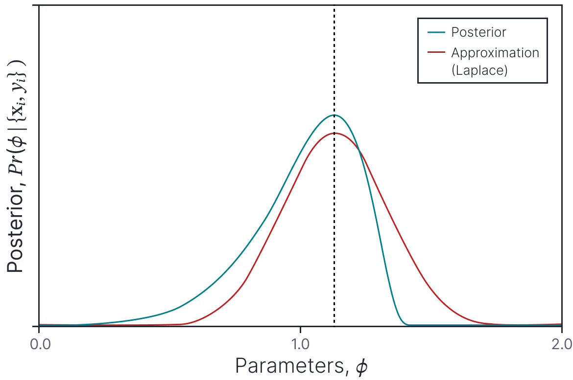
Figure 5. Laplace approximation. A probability density (cyan curve) is approximated by a normal distribution (orange curve). The mean of the normal (and hence the peak) is chosen to coincide with the peak of the original pdf. The variance of the normal is chosen so that its second derivatives at the mean match the second derivatives of the original pdf at the peak. The quality of this approximation depends on the degree to which the original pdf is similar to a normal.
In its most straightforward form, this is not practical for neural networks (the covariance matrix would be too large to represent). However, Ritter et al. (2018) developed a scalable Laplace approximation for neural networks using a Kronecker product of much smaller matrices. This is tractable, but the Laplace approximation still has the disadvantage that it is extremely local; it only relies on information at the MAP solution, it does not capture multiple modes in the distribution, and may not even characterize the shape of the MAP mode well.
SWAG (Maddox et al., 2019) adapts an earlier technique called stochastic weight averaging or SWA (Izmailov et al., 2018) to compute a different Gaussian approximation. SWA trained in a conventional way but used a learning rate schedule that decays to a relatively high constant learning rate. This causes the SGD solution to bounce around rather than to converge and hence sample the posterior across a local region near the true solution. The SWA solution is a new model where the weights are the average of the weights of the sample models.
SWAG (the `G’ stands for Gaussian) extended this by also describing the covariance of the sampled weights (using a low-rank plus diagonal parameterization). Once we have the mean and covariance of the weights, we can draw as many weight samples as we want and use these to perform inference using equation 10 (figure 6a-b). This has the advantage that it is not only based on the properties of the loss function at the MAP solution. However, it still only describes one mode of this distribution.
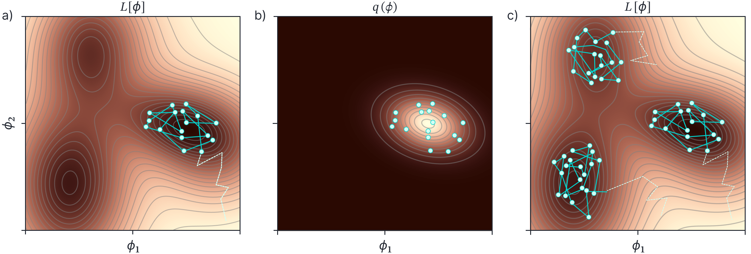
Figure 6. SWAG and MultiSWAG. a) SWAG uses relatively high learning rate that causes the estimated parameters (cyan path) to bounce around the minimum of this loss function. After a burn in period (dashed part of path), the parameters are collected at each update (cyan points). b) A Gaussian $q(\boldsymbol\phi)$ is fit to these points, and we can draw as many samples as we want from this Gaussian to perform inference. c) Multi-SWAG repeats this procedure several times, so that we also sample different minima in the loss function.
Deep ensembles and MultiSWAG
Examination of equation 10 reveals that the Bayesian prediction resembles combining models in an ensemble. Lakshminarayanan et al. (2017) created ensembles of deep neural networks; they retrain a model multiple times to find different solutions starting from different initializations and average together the predictions of the models. This was considered by some to be an approximation of the Bayesian approach. However, others disagree with this notion and consider the ensemble to be a different kind of “combination” model that could itself be subjected to a Bayesian treatment (e.g., see Minka, 2000).
Regardless of the philosophical disagreements, deep ensembles have the advantage that they capture information about different modes of the distribution. However, they do not capture the shape of each mode. Wilson and Izmailov (2020) introduced MultiSWAG (figure 6c) which combines the benefits of SWAG (characterizing the loss around a particular mode) with deep ensembles (combining point estimates from different mode). They combine different SWAG solutions generated from different initializations to form a Gaussian mixture posterior which can then be sampled from. Interestingly, they showed that double descent is not observed with MultiSWAG. This is presumably because errors induced when the model has barely enough parameters and must contort itself to fit the data average out across the different samples.
Variational approximation
Recall that our goal was to compute the posterior distribution over the parameters $\boldsymbol\phi$ given the training data set $\{\mathbf{x}_{i},\mathbf{y}_{i}\}$ using Bayes’s rule:
\begin{eqnarray}\label{eq:Bayes3_Bayes2b}
Pr(\boldsymbol\phi | \{\mathbf{x}_{i},\mathbf{y}_{i}\}) &=& \frac{\prod_{i=1}^{I} Pr(y_{i}|\mathbf{x}_{i},\boldsymbol\phi)Pr(\boldsymbol\phi)}{\int \prod_{i=1}^{I} Pr(y_{i}|\mathbf{x}_{i},\boldsymbol\phi)Pr(\boldsymbol\phi)d\boldsymbol\phi}.
\tag{12}
\end{eqnarray}
Unfortunately, for neural network models, there is generally no closed-form solution for this posterior distribution. In the previous section, we looked at methods that approximate the posterior with a set of samples. In this section, we consider methods that directly approximate the posterior with a simpler distribution (figure 1b).
To this end, we first choose a functional form for this variational distribution $q(\boldsymbol\phi)$. A typical choice is a normal distribution that is either spherical (so the uncertainty on each parameter is independent of all the others) or factorized (so, for example, the uncertainties of the weights at each layer are independent of the uncertainty of those at other layers). Other work models the distribution over each weight with a rank-1 parameterization (Dusenberry et al., 2020). Whichever choice we make, the variational distribution $q(\boldsymbol\phi|\boldsymbol\theta)$ will have parameters $\boldsymbol\theta$. For the normal distribution, this would be the mean and covariance.
To fit the variational distribution, we minimize the Kullback-Leibler divergence between the variational distribution $q(\boldsymbol\phi|\boldsymbol\theta)$ and the posterior $Pr(\boldsymbol\phi | \{\mathbf{x}_{i},\mathbf{y}_{i}\})$ as a function of the variational parameters $\boldsymbol\theta$:
\begin{eqnarray}
\hat{\boldsymbol\theta} &=&\mathop{argmin}_{\boldsymbol\theta}\biggl[D_{KL}\Bigl[q(\boldsymbol\phi|\boldsymbol\theta)\bigl\lVert Pr(\boldsymbol\phi | \{\mathbf{x}_{i},\mathbf{y}_{i}\})\Bigr]\biggr]\nonumber \\
&=&\mathop{argmin}_{\boldsymbol\theta}\Biggl[\int q(\boldsymbol\phi|\boldsymbol\theta) \log\biggl[\frac{q(\boldsymbol\phi|\boldsymbol\theta)}{Pr(\boldsymbol\phi | \{\mathbf{x}_{i},\mathbf{y}_{i}\})}\biggr]d\boldsymbol\phi\Biggr],
\tag{13}
\end{eqnarray}
where we have substituted in the expression for the Kullback-Leibler divergence in the second line. If we now introduce the expression for the posterior from Bayes’ rule (equation 12b):
\begin{eqnarray}\label{eq:Bayes3_variational}
\hat{\boldsymbol\theta}
&=&\mathop{argmin}_{\boldsymbol\theta}\Biggl[\int q(\boldsymbol\phi|\boldsymbol\theta) \log\Biggl[\frac{q(\boldsymbol\phi|\boldsymbol\theta)\int \prod_{i=1}^{I} Pr(y_{i}|\mathbf{x}_{i},\boldsymbol\phi)Pr(\boldsymbol\phi)d\boldsymbol\phi}{\prod_{i=1}^{I} Pr(y_{i}|\mathbf{x}_{i},\boldsymbol\phi)Pr(\boldsymbol\phi)}\Biggr]d\boldsymbol\phi\Biggr]\nonumber \\
&=& \mathop{argmin}_{\boldsymbol\theta}\Biggl[\int q(\boldsymbol\phi|\boldsymbol\theta)\Biggl( \log\Biggl[\frac{q(\boldsymbol\phi|\boldsymbol\theta)}{\prod_{i=1}^{I} Pr(y_{i}|\mathbf{x}_{i},\boldsymbol\phi)Pr(\boldsymbol\phi)}\Biggr] \nonumber \\
&& \hspace{4cm}+ \log\Biggl[\int\prod_{i=1}^{I} Pr(y_{i}|\mathbf{x}_{i},\boldsymbol\phi)Pr(\boldsymbol\phi)d\boldsymbol\phi\Biggr]\Biggr) d\boldsymbol\phi\Biggr]\nonumber \\
&=& \mathop{argmin}_{\boldsymbol\theta}\Biggl[\int q(\boldsymbol\phi|\boldsymbol\theta) \log\Biggl[\frac{q(\boldsymbol\phi|\boldsymbol\theta)}{\prod_{i=1}^{I} Pr(y_{i}|\mathbf{x}_{i},\boldsymbol\phi)Pr(\boldsymbol\phi)}\Biggr]d\boldsymbol\phi\Biggr],
\tag{14}
\end{eqnarray}
where we have dropped the second term (which was originally the denominator of Bayes’ rule) because it is independent of the parameters $\boldsymbol\phi$ of the model (which are integrated out) and so has no effect on the approximation. In this way, we sidestep the intractable term from Bayes’ rule.
Bayes by backprop
Blundell et al. (2015) proposed a method known as Bayes by backprop to optimize this criteron. They identify that the final loss function $L[\boldsymbol\theta]$ from equation 14 can equivalently be written as an expectation:
\begin{eqnarray}
L[\boldsymbol\theta] &=& \int q(\boldsymbol\phi|\boldsymbol\theta) \log\Biggl[\frac{q(\boldsymbol\phi|\boldsymbol\theta)}{\prod_{i=1}^{I} Pr(y_{i}|\mathbf{x}_{i},\boldsymbol\phi)Pr(\boldsymbol\phi)}\Biggr]d\boldsymbol\phi\nonumber \\&=& \mathbb{E}_{q(\boldsymbol\phi|\boldsymbol\theta)} \Biggl[\log\Biggl[\frac{q(\boldsymbol\phi|\boldsymbol\theta)}{\prod_{i=1}^{I} Pr(y_{i}|\mathbf{x}_{i},\boldsymbol\phi)Pr(\boldsymbol\phi)}\Biggr]\Biggr],
\tag{15}
\end{eqnarray}
and as such, it can be approximated by a set of $S$ samples $\{\boldsymbol\phi_{s}\}_{s=1}^{S}$ from $q(\boldsymbol\phi|\boldsymbol\theta)$:
\begin{equation}
L[\boldsymbol\theta] \approx \frac{1}{S} \log\Biggl[\frac{q(\boldsymbol\phi_s|\boldsymbol\theta)}{\prod_{i=1}^{I} Pr(y_{i}|\mathbf{x}_{i},\boldsymbol\phi_s)Pr(\boldsymbol\phi_s)}\Biggr]
\tag{16}
\end{equation}
In principle, we could draw samples (or even a single sample) to estimate the loss function and compute the derivatives with respect to $\boldsymbol\theta$ using backpropagation (figure 7a–b). Unfortunately, it is difficult to backpropagate through the sampling step, and so we use the reparameterization trick (see chapter 17 of Prince, 2023). Here, we move the underlying random variable $\boldsymbol\epsilon$ into a separate branch of the computational network (figure 7c). For example, if the variational distribution was normal we might have $\boldsymbol\theta=\{\boldsymbol\mu, \boldsymbol\Sigma\}$ and we could compute the samples as:
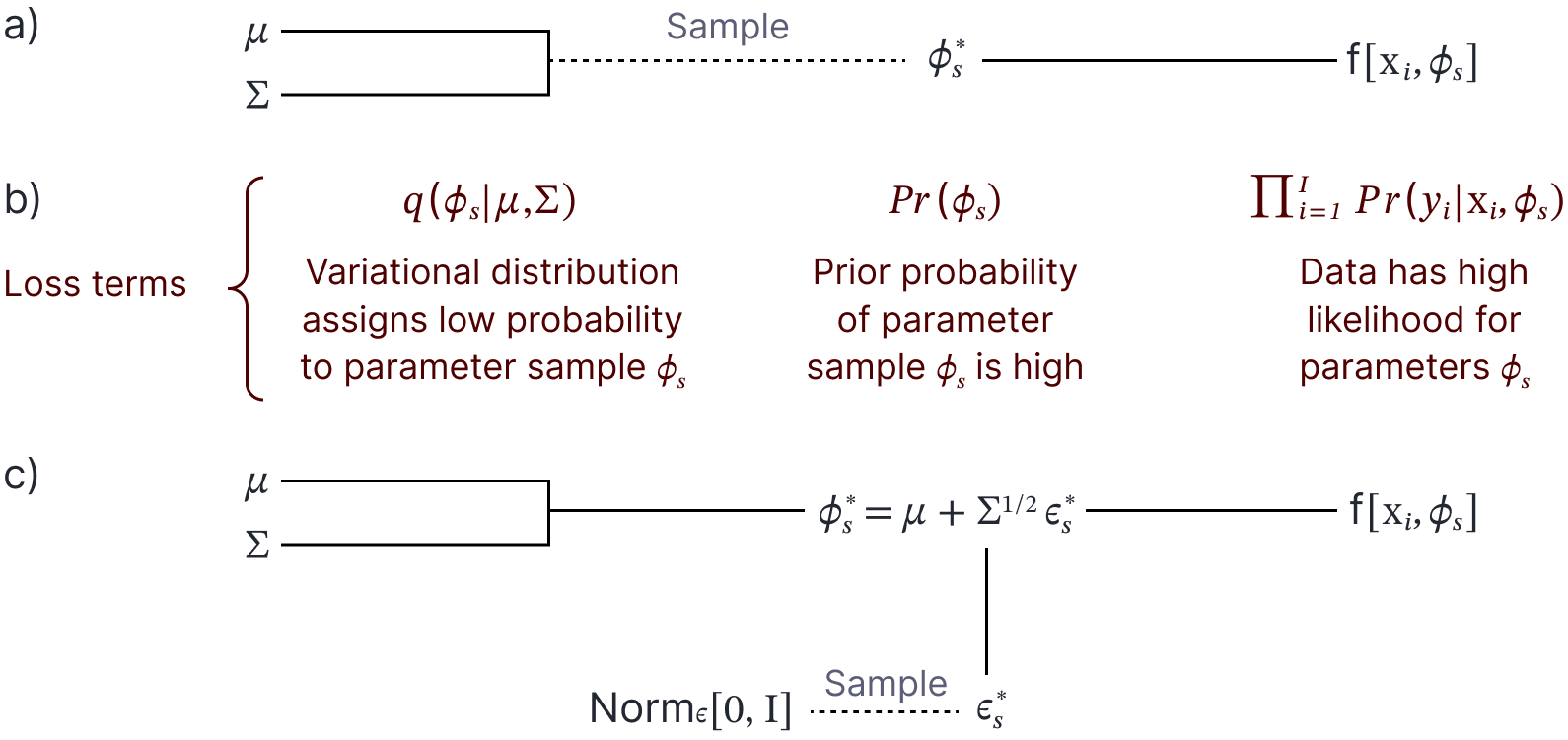
Figure 7. Bayes by backprop. a) Sample parameters $\boldsymbol\phi_s$ are drawn from the variational distribution (here a Gaussian with mean $\boldsymbol\mu$ and covariance $\boldsymbol\Sigma$). The sample parameters are then used in the model $\mbox{f}[\mathbf{x}_i, \boldsymbol\phi_{s}]$. b) The loss function contains three terms (the probability of the parameter sample under the variational distribution, the prior probability of the parameter sample, and the likelihood of the data under the model with the sample parameters). The first of these terms prevents the distribution collapsing to a single point at the MAP solution. We improve the variational parameters $\boldsymbol\mu$ and $\boldsymbol\Sigma$ by backpropagating through this computational graph. However, it is challenging to backpropagate through the sampling stage. c) To this end we use the $\textit{reparameterization trick}$ in which the sampling is removed from the main computational graph.
\begin{equation}
\boldsymbol\phi_{s} = \boldsymbol\mu +\boldsymbol\Sigma^{1/2} \boldsymbol\epsilon_{s}
\tag{17}
\end{equation}
where $\boldsymbol\epsilon_{s}$ is drawn from a standard normal distribution.
Inference
At the end of this process, we have an approximation $q(\boldsymbol\phi|\boldsymbol\theta)$ over the model parameters $\boldsymbol\phi$. To make a prediction, we must compute the integral:
\begin{eqnarray}
Pr\bigl(y^*|\mathbf{x}^*,\{\mathbf{x}_{i},\mathbf{y}_{i}\}\bigr) &=& \int Pr\bigl(y^*|\mathbf{x}^*,\boldsymbol\phi\bigr) Pr\bigl(\boldsymbol\phi|\{\mathbf{x}_{i},\mathbf{y}_{i}\}\bigr) d\boldsymbol\phi\nonumber \\
&\approx & \int Pr\bigl(y^*|\mathbf{x}^*,\boldsymbol\phi\bigr) q(\boldsymbol\phi|\boldsymbol\theta) d\boldsymbol\phi.
\tag{18}
\end{eqnarray}
In general, this can still not be done in closed form. If the variational distribution is Gaussian, we could make a prediction based on the mean alone. This is generally better than if we had used a conventional maximum likelihood scheme as the mean has been computed taking into account the uncertainty in the parameters. A better approach is to draw samples from $q(\boldsymbol\phi|\boldsymbol\theta)$ and take the average of the predictions. This also provides a measure of uncertainty on the predictions.
Wu et al. (2018) improved on these methods by inducing a method for inference that can predict uncertainty on the outputs without sampling. They assume a variational distribution with a structured Gaussian form where parameters in different layers are independent. Then they note that the uncertain weights induce uncertainty in the preactivations at a layer; this uncertainty is propagated through the non-linearities by approximating the resulting distribution by another Gaussian and estimating the moments. In this way, the uncertainty can be propagated through the network to the final weights. This is very similar to the calculation in neural network Gaussian processes (see part VII of this series).
Monte Carlo dropout
Dropout (Hinton et al., 2012) is a regularization technique that randomly clamps a subset (typically 50%) of hidden units to zero at each iteration of SGD. This makes the network less dependent on any given hidden unit and encourages the weights to have smaller magnitudes so that the change in the function due to the presence or absence of the hidden unit is reduced (figure 8).
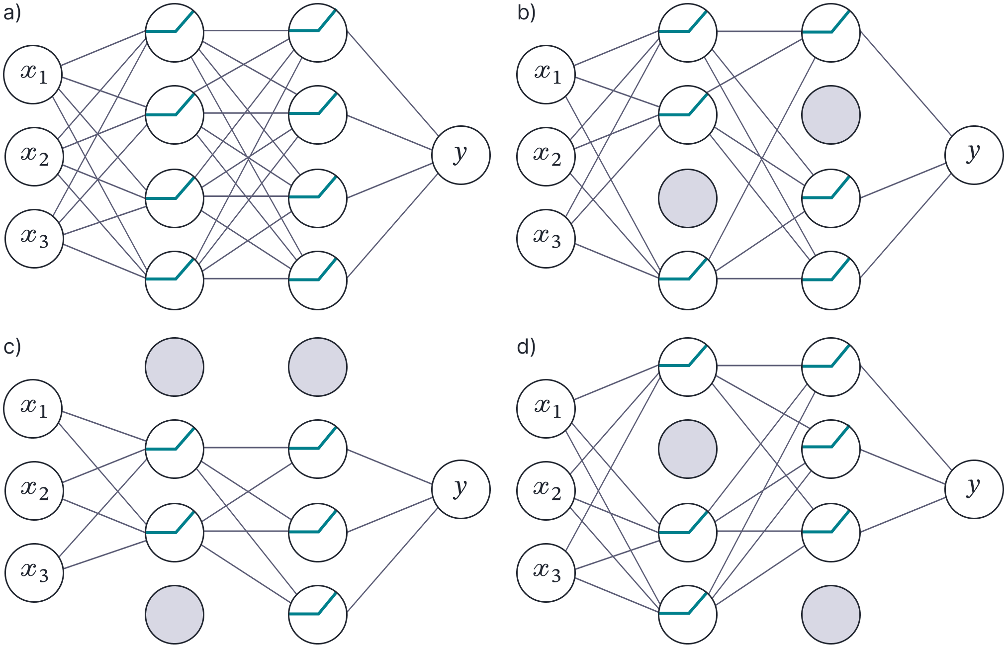
Figure 8. Dropout. a) Original network. b–d) At each training iteration, a random subset of hidden units is clamped to zero (gray nodes). The result is that the incoming and outgoing weights from these units have no effect, so we are training with a slightly different network each time.
Gal and Gharamani (2015) showed that dropout could be interpreted as a variational approximation where the posterior over the paramemters $\boldsymbol\phi$ is given by:
\begin{equation}
\boldsymbol\phi \sim \boldsymbol\mu \cdot \mathbf{Bern}[p]
\tag{19}
\end{equation}
where $\boldsymbol\mu$ is a variational parameter, and $\mathbf{Bern}[\lambda]$ returns a random vector of ones and zero drawn from a Bernoulli distribution with parameter $\lambda$. This is not a true Bayesian method though, because the posterior distribution over the parameters doesn’t become sharper as the observed data increases.
Conclusion
This blog has considered Bayesian learning for neural networks from the parameter perspective. These Bayesian neural networks are attractive because they can account for many different explanations of the data. Unfortunately, the posterior distribution over the parameters is intractable and hence we must approximate it using samples, a simpler distribution (the variational approach) or some combination of the two approaches.
Despite these drawbacks, we’ve seen that Bayesian neural networks can yield better performance than standard training and also provide measures of uncertainty. Further information about Bayesian learning for neural networks can be found in the review papers of Margirs and Iosifidis (2023) and Arbel et al. (2023).
In part VII of this series we will consider the Bayesian approach to neural networks from the function perspective. We will see that this is tractable for infinite width networks, but inference scales polynomially with the number of data points, so they are are only practical for relatively small datasets.
Join RBC Borealis!
Are you aspiring to build a career in AI and ML research? We have several student programs and full-time opportunities.
View open roles