
In part IV and part V of this series of blogs we investigated Bayesian machine learning from the parameter and function perspectives, respectively. We saw that these two viewpoints yield the same results for a linear regression model. In part VI we saw that Bayesian learning in neural networks from a parameter perspective is intractable; to make progress we are forced to rely on a variational approximation or sampling strategies.
In part VII (this final blog), we apply Bayesian machine learning to neural networks from the function space perspective. Happily, we will see that this is tractable; we can make exact predictions from a deep neural network with infinite width, and these are accompanied by estimates of uncertainty. These models are referred to as neural network Gaussian processes.
This blog is accompanied by a CoLab notebook that recreates most of the figures.
Random shallow networks
Throughout this blog, we will consider a neural network $\hat{y} = \mbox{f}[x, \boldsymbol\phi]$ with a single univariate input $x\in\mathbb{R}$, a single output $\hat{y}\in\mathbb{R}$ and parameters $\boldsymbol\phi$. The network is defined as:
\begin{eqnarray}
h_{d} &=& \mbox{ReLU}\Bigl[\beta_{0d} + \omega_{0d}x\Bigr] \nonumber\\
\mbox{f}[x,\boldsymbol\phi] &=& \beta_{1} + \sum_{d=1}^{D}\frac{\omega_{1d}h_{d}}{\sqrt{D}},
\tag{1}
\end{eqnarray}
where $h_{d}$ is the $d^{th}$ of $D$ hidden units and $\mbox{ReLU}[a] = \max\bigl[0,a\bigr]$ is the rectified linear unit activation function. The parameters $\boldsymbol\phi=\{\beta_{0\bullet},\omega_{0\bullet},\beta_{1},\omega_{1\bullet} \}$ comprise the biases $\beta_{0d}$ and weights $\omega_{0d}$ that are used to compute the preactivations $\beta_{0d} + \omega_{0d}x$, and the bias $\beta_{1}$ and weights $\omega_{1d}$ that recombine the activations $h_{d}$ at the hidden units to create the output. This is a standard neural network except for the normalizing factor $1/\sqrt{D}$ which ensures that the magnitude of the network output stays roughly the same as we change the number of hidden units $D$.
Let’s place Gaussian priors over the biases and weights with mean zero and variance $\sigma^2_{\beta}$ and $\sigma^2_{\omega}$ respectively:
\begin{eqnarray}
\beta_{0d}, \beta_1 &\sim& \mbox{Norm}\Bigl[0,\sigma^2_{\beta}\Bigr]\nonumber\\
\omega_{0d}, \omega_{1d} &\sim& \mbox{Norm}\Bigl[0,\sigma^2_{\omega}\Bigr].
\tag{2}
\end{eqnarray}
We can now draw random neural networks by sampling from these priors. Each preactivation (figure 1a) is a linear function of the data and each activation (figure 1b) is a clipped linear function. The output of each neural network (which is a weighted sum of the constituent activations) is a more complicated non-linear function. Note that the functions are non-stationary. The variance of the functions becomes larger as $x\rightarrow\pm\infty$. They also tend to change in complex ways near the origin but become linear as $x\rightarrow\pm\infty$; at some point, the joint in the last ReLU function is passed and after this the curve continues on a constant trajectory.
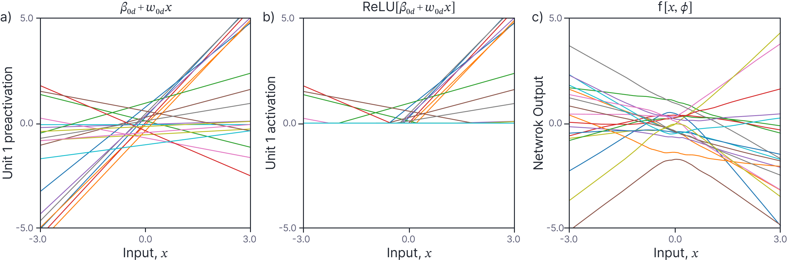
Figure 1. Random draws from neural networks with $\sigma^2_{\beta}=0.5$ and $\sigma^2_{\omega}=1.0$ and $D=1000$ hidden units. a) The preactivations at the $d^{th}$ hidden unit are linear functions of the data with y-offset $\beta_{0d}$ and slope $\omega_{0d}$. b) The activations at the $d^{th}$ hidden unit are lines that are truncated at zero. c) Each neural network output is a random weighted combination of the $D=1000$ activations plus a further random bias.
Shallow networks as Gaussian processes
Now that we have defined a neural network function and a prior over the parameters, we will investigate the joint probability distributions for the pre-activations, activations, and the outputs at two different points $x$ and $x’$. We will show that the pre-activations and outputs are normally distributed but that the activations have a more complex distribution. We’ll derive expressions for the mean and covariance of all three quantities.
The conclusion of this investigation will be that:
- The outputs of a randomly initialized neural network at any two points $x$ and $x’$ are jointly normally distributed and their mean and covariance can be computed in closed form as a function of $x$ and $x’$.
- It follows that this is a Gaussian process, and we can use this Gaussian process to make predictions when conditioned on some observed data.
Covariance of preactivations
Figure 2a shows the preactivations from the first hidden unit of twenty randomly generated neural networks. Consider two points $x=1.0$ and $x’=1.5$ (vertical dashed lines). Figure 2b shows a scatterplot of the preactivations at these two points for 100 randomly generated networks. The scatterplot suggests that the preactivations at these points are normally distributed with zero mean. Indeed, figures 2c-f suggests that the preactivations at any two points $x$ and $x’$ are normally distributed with zero mean and a covariance that depends on $x$ and $x’$.
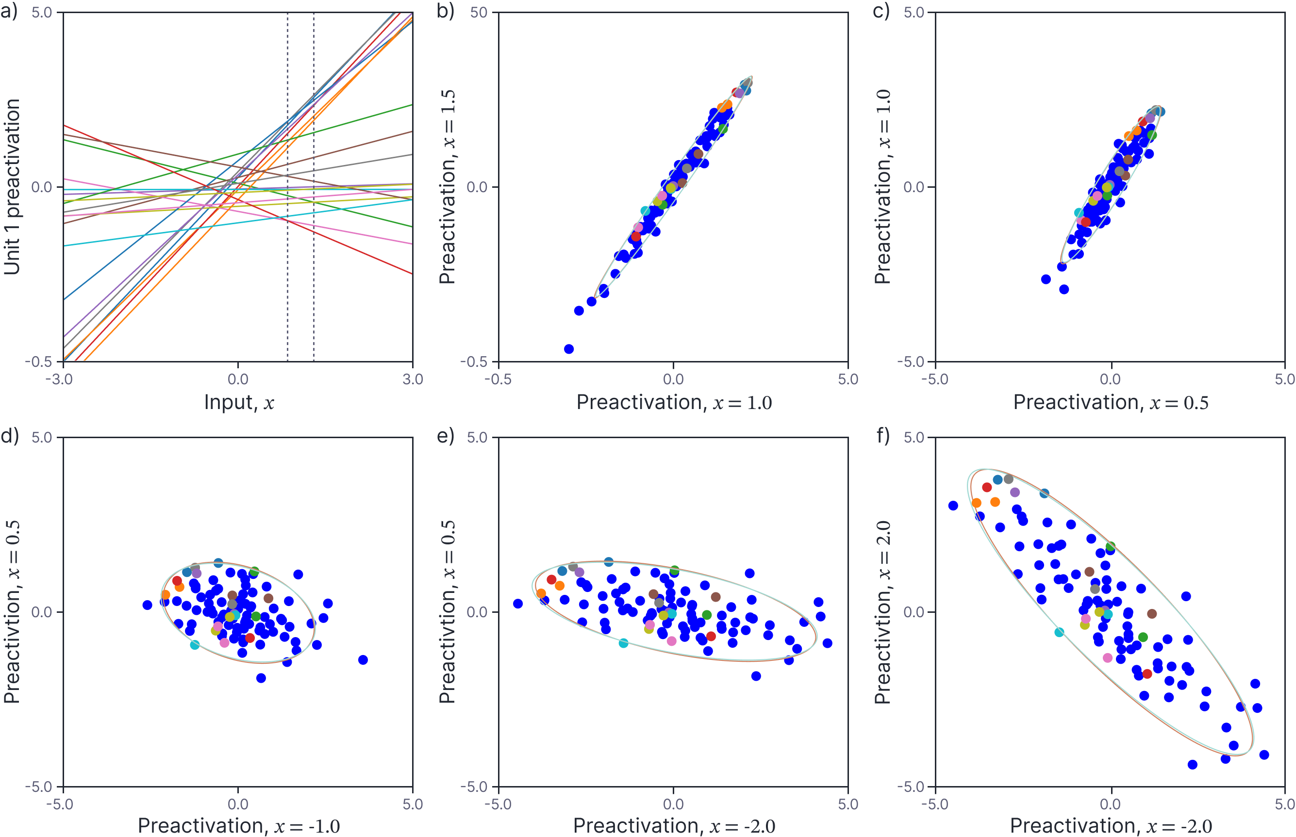
Figure 2. Covariance of preactivations. a) The preactivations at the first neuron for twenty different randomly generated neural networks. Consider two points $x=1.0$ and $x’=1.5$ (vertical dashed lines). b) Scatterplot of preactivations at these two points for 100 randomly generated networks (the first twenty are colored as in panel a). The preactivations are normally distributed with mean zero and an empirical covariance indicated by the orange ellipse (computed from 1000 pairs). This is very close to (and mostly obscured by) the predicted covariance (cyan ellipse). c-f) Scatterplots, empirical covariance, and predicted covariance for four other pairs of values $x$ and $x’$ (each would correspond to two different vertical dashed lines in panel a).
In fact, these distributions must be normal as they can be construed as linear transformations of the normally distributed weights $\beta_{0d}$ and $\omega_{0d}$:
\begin{equation}
\begin{bmatrix}
\beta_{0d}+\omega_{0d}x\\
\beta_{0d}+\omega_{0d} x’
\end{bmatrix} = \begin{bmatrix}1 & x \\ 1 & x’\end{bmatrix}\begin{bmatrix}\beta_{0d}\\\omega_{0d}\end{bmatrix},
\tag{3}
\end{equation}
and it’s straightforward to compute the mean and covariance of the two points. The mean (expected value) of the preactivations is zero:
\begin{eqnarray}
\mathbb{E}_{\beta_{0d},\omega_{0d}}\Bigl[\beta_{0d}+\omega_{0d} x\Bigr] &=& \mathbb{E}\Bigl[\beta_{0d}\Bigr] + \mathbb{E}\Bigl[\omega_{0d}\Bigr] \cdot x\nonumber \\
&=& 0 + 0\cdot x = 0,
\tag{4}
\end{eqnarray}
where we have used standard rules for manipulating expectations (see Appendix C.2 of this book). The calculation is the same for the second point $x’$.
The covariance matrix of the two quantities $a$ and $a’$ is defined as:
\begin{eqnarray}
\mbox{Cov}[a,a’] = \mathbb{E}\left[\begin{bmatrix}a-\mathbb{E}[a]\\a’-\mathbb{E}[a’]\end{bmatrix}\begin{bmatrix}a-\mathbb{E}[a]\\a’-\mathbb{E}[a’]\end{bmatrix}^T\right].
\tag{5}
\end{eqnarray}
Substituting in $a= \beta_{0d}+\omega_{0d} x$ and $a’= \beta_{0d}+\omega_{0d} x’$ and noting that their expectations are both zero, we get:
\begin{eqnarray}
\mbox{Cov}\Bigl[\beta_{0d}+\omega_{0d} x,\beta_{0d}+\omega_{0d} x’\Bigr] &=&\nonumber \mathbb{E}\left[ \begin{bmatrix} \beta_{0d}+\omega_{0d} x \\ \beta_{0d}+\omega_{0d} x’\end{bmatrix}\begin{bmatrix} \beta_{0d}+\omega_{0d} x \\ \beta_{0d}+\omega_{0d} x’ \end{bmatrix}^T\right].
\end{eqnarray}
Taking the top-left element of this $2\times 2$ matrix first, we get:
\begin{eqnarray}
\mathbb{E}\Bigl[\bigl(\beta_{0d}+\omega_{0d} x\bigr)\bigl(\beta_{0d}+\omega_{0d} x,\bigr)\Bigr] &=& \mathbb{E}\Bigl[\beta_{0d}^2+ 2\beta_{0d}\omega_{0d}x + \omega_{0d}^2x^2 \Bigr]\nonumber \\
&=& \mathbb{E}\Bigl[\beta_{0d}^2\Bigr] + \mathbb{E}\Bigl[2\beta_{0d}\omega_{0d}x\Bigr] + \mathbb{E}\Bigl[\omega_{0d}^2x^2 \Bigr]\nonumber\\
&=& \sigma^{2}_{\beta} + 0 + \sigma^2_\omega x^2\nonumber \\
&=& \sigma^{2}_{\beta} + \sigma^2_\omega x^2.
\tag{6}
\end{eqnarray}
Proceeding in the same way for the other three entries, we find that the covariance of the preactivations is given by:
\begin{eqnarray}\label{eq:NNGP_preactivation_cov}
\mbox{Cov}\Bigl[\beta_{0d}+\omega_{0d} x,\beta_{0d}+\omega_{0d} x’\Bigr] &=& \begin{bmatrix} \sigma^{2}_{\beta}+\sigma^2_\omega x^2&\sigma^{2}_{\beta}+\sigma^2_\omega xx’\\\sigma^{2}_{\beta}+\sigma^2_\omega xx’&\sigma^{2}_{\beta}+\sigma^2_\omega x’^2\end{bmatrix} \nonumber\\
&=& \sigma^{2}_{\beta}+\sigma^2_\omega\begin{bmatrix}x\\x’\end{bmatrix}\begin{bmatrix}x&x’\end{bmatrix}.
\tag{7}
\end{eqnarray}
Panels b-e) of figure 2 show the empirically observed covariances of 1000 random neural networks each of which has 1000 hidden units (orange ellipse), and the predicted covariance as given by equation 7 (cyan ellipse). These are almost identical.
Covariance of activations
Now let’s consider what happens when we pass these distributions through the ReLU activation function. Figure 3a shows the activations from the first hidden unit of twenty randomly generated neural networks as a function of the input. Again, consider two points $x=1.0$ and $x’=1.5$ (vertical dashed lines). Figure 3b shows the scatterplot of these two values, and the remaining panels show scatterplots of other pairs $\{x,x’\}$ of values. Clearly, these distributions are not Gaussian. This is unsurprising; for example, if you consider the last panel which plots the activation values for $x=2.0$ and $x’=-2.0$, one value is taken from the left-hand side of figure 3a and the other from the right-hand side and hence one or the other is almost always clipped to zero.
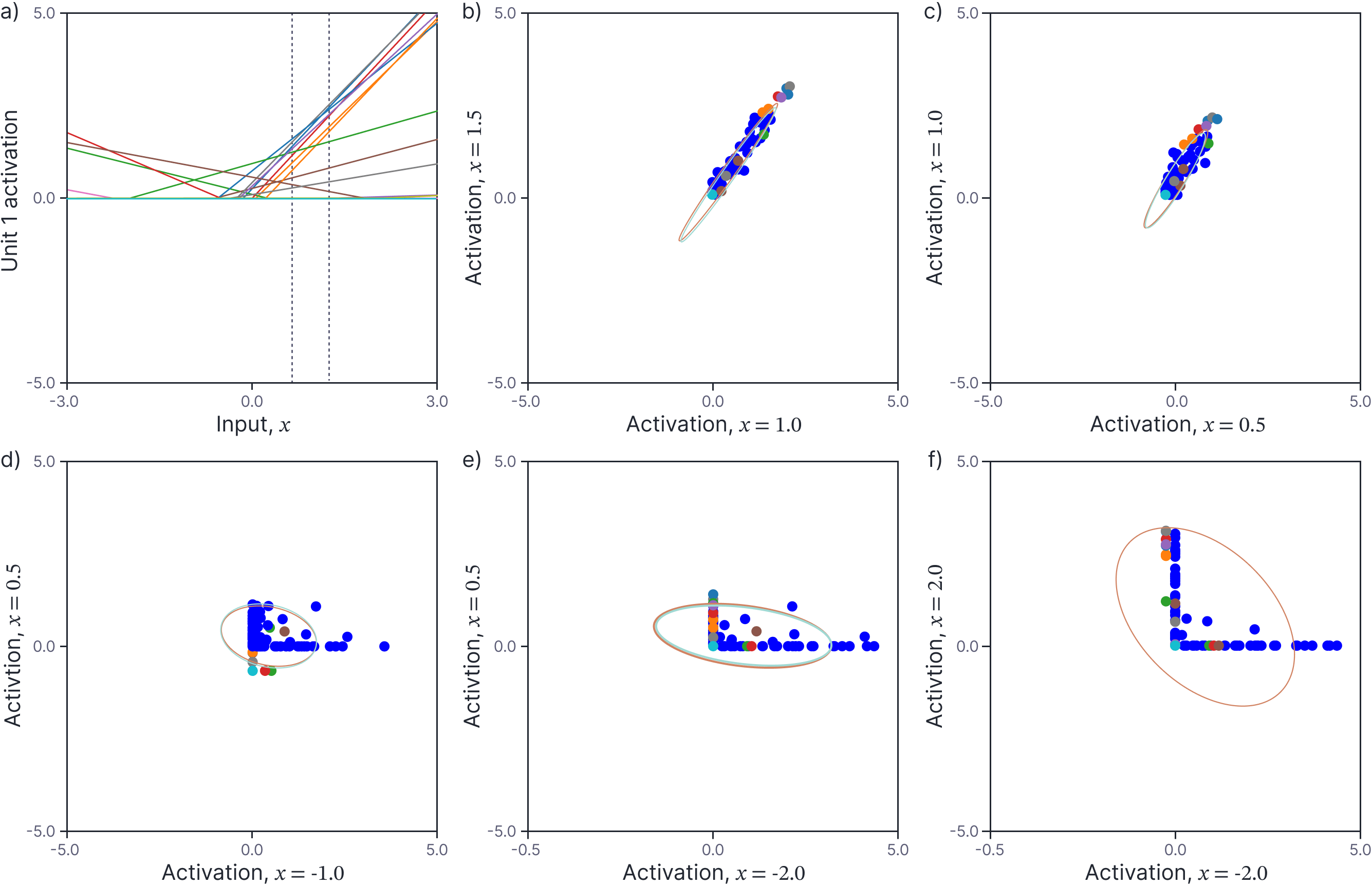
Figure 3. Covariance of activations. a) The activations at the first neuron for twenty different randomly generated neural networks. Consider two points $x = 1.0$ and $x^′ = 1.5$ (vertical dashed lines). b) Scatterplot of activations at these two points for 100 randomly generated networks (the first twenty are colored as in panel a). The activations are not normally distributed but have an empirical mean and covariance indicated by the orange ellipse (computed from 1000 pairs). This is very close to (and mostly obscured by) the predicted covariance (cyan ellipse). c-f) Scatterplots, empirical covariance, and predicted covariance for four other pairs of values $x$ and $x^′$ (each would correspond to two different vertical dashed lines in panel a).
Although these distributions are not Gaussian, we can still compute their mean and covariance using the following two relations:
Relation 1: To compute the mean, we use the relation that for $z\sim\mbox{Norm}_z[\mu, \sigma^2]$:
\begin{eqnarray}
\mathbb{E}_{z}\bigl[\mbox{ReLU}[z]\bigr] &=& \sigma \cdot \mbox{Norm}_{\mu/\sigma}[0,1] + \mu\cdot \mbox{cnorm}\left[\frac{\mu}{\sigma}\right],
\tag{8}
\end{eqnarray}
where $\mbox{cnorm}[z]$ is the cumulative normal distribution. This relation is proven at the end of this document.
Relation 2: To compute the covariance of the activations we use the (non-obvious) result that if:
\begin{equation}
\mathbf{z} = \begin{bmatrix}z_{1}\\z_{2}\end{bmatrix} \sim \mbox{Norm}_{\mathbf{z}}\left[
\begin{bmatrix}0\\0\end{bmatrix},
\begin{bmatrix}\sigma^2_{11} & \sigma^2_{12}\\ \sigma^2_{21} & \sigma^2_{22} \end{bmatrix}^{\hspace{-0.12cm}\color{white}’} \right],
\tag{9}
\end{equation}
then:
\begin{eqnarray}
\mathbb{E}_{\mathbf{z}}\Bigl[\mbox{ReLU}[z_{i}]]\cdot \mbox{ReLU}[z_{j}]\Bigr]
&=& \frac{\sigma_{11}\sigma_{22}\left(\cos[\theta]\cdot \Bigl(\pi -\theta\Bigr)+\sin[\theta]\right)}{2\pi},
% \nonumber \\
% \mathbb{E}\Bigl[\mathbb{I}[z_{i}>0]\cdot \mathbb{I}[z_{j}>0]\Bigr]
% &=& \frac{\pi-\theta}{2\pi}
\tag{10}
\end{eqnarray}
where
\begin{equation}
\theta = \arccos\left[\frac{\sigma^2_{12}}{\sigma_{11}\cdot\sigma_{22}}\right].
\tag{11}
\end{equation}
See Cho and Saul, 2009 and Golikov et al. (2022) for proofs of this relation.
Applying the first relation the expected value of the activations $h_{d}$ at the hidden units is:
\begin{eqnarray}
\mathbb{E}\bigl[h_{d}\bigr]&=& (\sigma^2\beta+\sigma^2_\omega x ^2) \cdot \mbox{Norm}_{0/(\sigma^2\beta+\sigma^2_\omega x^2)}[0,1] + 0 \cdot \mbox{cnorm}\left[\frac{0}{\sigma^2\beta+\sigma^2_\omega x ^2 }\right]\nonumber \\
&=& \frac{\sigma^2\beta+\sigma^2_\omega x ^2 }{\sqrt{2\pi}},
\tag{12}
\end{eqnarray}
where the expectation is taken over the random parameters $\beta_{0d}, \omega_{0d}$ and we have used the fact that the mean of the preactivations is zero and the covariance is given by equation 7.
Applying the second relation, the off-diagonal terms in the covariance matrix are given by:
\begin{eqnarray}
\mathbb{E}\bigl[h_d h_d’\bigr]
= \frac{\sqrt{(\sigma^{2}_{\beta}+\sigma^2_\omega x^2)( \sigma^{2}_{\beta}+\sigma^2_\omega x’^2)}\Bigl(\cos[\theta]\cdot \bigl(\pi -\theta\bigr)+\sin[\theta]\Bigr)}{2\pi},
\tag{13}
\end{eqnarray}
where:
\begin{equation}
\theta = \arccos\left[\frac{\sigma^{2}_{\beta}+\sigma^2_\omega xx’}{\sqrt{(\sigma^{2}_{\beta}+\sigma^2_\omega x^2)( \sigma^{2}_{\beta}+\sigma^2_\omega x’^2)}}\right],
\tag{14}
\end{equation}
and the diagonal terms (calculated by using the same formula with $x=x’$) simplify to:
\begin{equation}
\mathbb{E}\bigl[h^2 \bigr] = \frac{\sigma^{2}_{\beta}+\sigma^2_\omega x^2}{2}.
\tag{15}
\end{equation}
Figure 3b-d depict the predicted mean and covariance of the first hidden unit activation with a cyan ellipse. The empirical mean and covariance of the activations computed from 1000 random networks is shown as an orange ellipse. As expected, these are in close agreement.
Covariance of outputs
Finally, let’s consider the mean and covariance of the network output $\mbox{f}[x, \boldsymbol\phi]$ for input points $x$ and $x’$. Figure 4a depicts the network output for twenty randomly drawn networks as a function of the input $x$. For a final time, we consider two points $x=1.0$ and $x’=1.5$ (vertical dashed lines). Figure 4b shows a scatterplot of the function outputs for these two inputs. The plot suggests that the output are normally distributed with mean zero. Figures 4c-f demonstrate that the covariance depends on the particular choice of input points; in general the variance increases as the points move away from zero, and their correlation decreases as they grow further apart from one another.
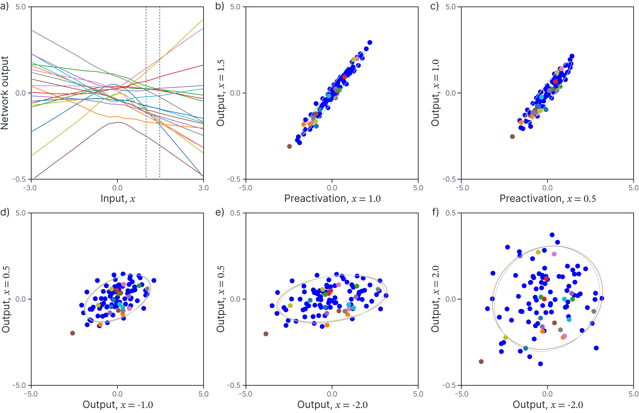
Figure 4. Covariance of network outputs. a) The outputs at the first neuron for twenty different randomly generated neural networks. Consider two points $x = 1.0$ and $x^′ = 1.5$ (vertical dashed lines). b) Scatterplot of outputs at these two points for 100 randomly generated networks (the first twenty are colored as in panel a). The outputs are normally distributed with mean zero and have empirical mean and covariance indicated by the orange ellipse (computed from 1000 pairs). This is very close to (and mostly obscured by) the predicted covariance (cyan ellipse). c-f) Scatterplots, empirical covariance, and predicted covariance for four other pairs of values $x$ and $x^′$ (each would correspond to two different vertical dashed lines in panel a).
Let’s now find expressions for the mean and covariance of the network outputs. Recall that the network definition was:
\begin{eqnarray}
h_{d} &=& \mbox{ReLU}\Bigl[\beta_{0d} + \omega_{0d}x\Bigr] \nonumber\\
\mbox{f}[x,\boldsymbol\phi] &=& \beta_{1} + \sum_{d=1}^{D}\frac{\omega_{1d}h_{d}}{\sqrt{D}}.
\tag{16}
\end{eqnarray}
Let’s first consider the terms $\omega_{1d}h_{d}/\sqrt{D}$.
\begin{eqnarray}
\mathbb{E}\left[\frac{\omega_{1d}h_{d}}{\sqrt{D}}\right] &=& \frac{1}{\sqrt{D}}\mathbb{E}\bigl[\omega_{1d}h_{d}\bigr]\nonumber \\
&=& \frac{1}{\sqrt{D}}\mathbb{E}\bigl[\omega_{1d}\bigr]\cdot \mathbb{E}\bigl[h_{d}\bigr]\nonumber\\
&=& \frac{1}{\sqrt{D}}0\cdot \mathbb{E}\bigl[h_{d}\bigr] = 0,
\tag{17}
\end{eqnarray}
where the transition from the first line to the second follows because $\omega_{1d}$ and $h_{d}$ are independently distributed (see Appendix C.2 of this book).
Now let’s consider the covariance:
\begin{eqnarray}
\mathbb{E}\left[\frac{\omega_{1d}h_{d}}{\sqrt{D}}\frac{\omega_{1d}h’_{d}}{\sqrt{D}}\right] &=& \frac{1}{D}\cdot\mathbb{E}\bigl[\omega^2_{1d}h_{d}h’_{d}\bigr]\nonumber \\
&=& \frac{1}{D}\cdot\mathbb{E}\bigl[\omega^2_{1d}\bigr]\mathbb{E}\bigl[h_{d}h’_{d}\bigr]\nonumber \\
&=& \frac{\sigma^2_{\omega}}{D}\cdot \mathbb{E}\bigl[h_{d}h’_{d}\bigr],
\tag{18}
\end{eqnarray}
where we computed the $\mathbb{E}[h_{d}h’_{d}]$ in the previous section. Finally, let’s consider the mean and covariance of the network output $\mbox{f}[x,\boldsymbol\phi] = \beta_{1} + \sum_{d=1}^{D}\omega_{1d}h_{d}/\sqrt{D}$. By inspection, we can see that:
\begin{eqnarray}
\mathbb{E}\Bigl[\mbox{f}[x,\boldsymbol\phi]\Bigr] &=& 0 \nonumber \\
\mathbb{E}\Bigl[\mbox{f}[x,\boldsymbol\phi], \mbox{f}[x’,\boldsymbol\phi]\Bigr] &=& \sigma^2_{\beta}+ \sigma^2_{\omega} \cdot \mathbb{E}\bigl[h_{d}h’_{d}\bigr],
\tag{19}
\end{eqnarray}
where the first relation follows because every term that is summed has mean zero, and the second term follows because we are summing independent quantities. Notably, the output is formed from a sum of $D$ independently distributed terms and so by the central limit theorem it will be normally distributed.
Figure 4b-d depict the predicted mean and covariance of the network output as computed by this method with a cyan ellipse. The empirical mean and covariance of the activations computed from 1000 random networks is shown as an orange ellipse. Once more, these are in close agreement.
Neural network Gaussian processes
In the previous section we showed that if we put Gaussian priors on the weights and biases of a shallow network, the joint probability distribution of the network outputs corresponding to inputs $x$ and $x’$ is a mean-zero Gaussian, and that we can compute the covariance of this Gaussian in closed form. As such, it is a type of Gaussian process, and we can apply the techniques of part V of this series of blogs. This model is termed a neural network Gaussian process and was first developed by Neal (1996).
Kernel
The kernel $\mathbf{K}[\mathbf{X}, \mathbf{X}]$ of the neural network Gaussian process is a $I\times I$ matrix where each position corresponds to a pair of the $I$ data points in $\mathbf{X}=[x_1, x_2, \ldots x_{I}]$, so position $(i,j)$ contains a value $\mbox{k}[x_{i},x_{j}] = \mathbb{E}\bigl[\mbox{f}[x_i,\boldsymbol\phi], \mbox{f}[x_j,\boldsymbol\phi]\bigr]$. The kernel is a function of the hyperparameters $\sigma^2_{\beta}$ and $\sigma^2_{\omega}$. Figure 5 visualizes the kernel for equally spaced points, as we vary these hyperparameters.
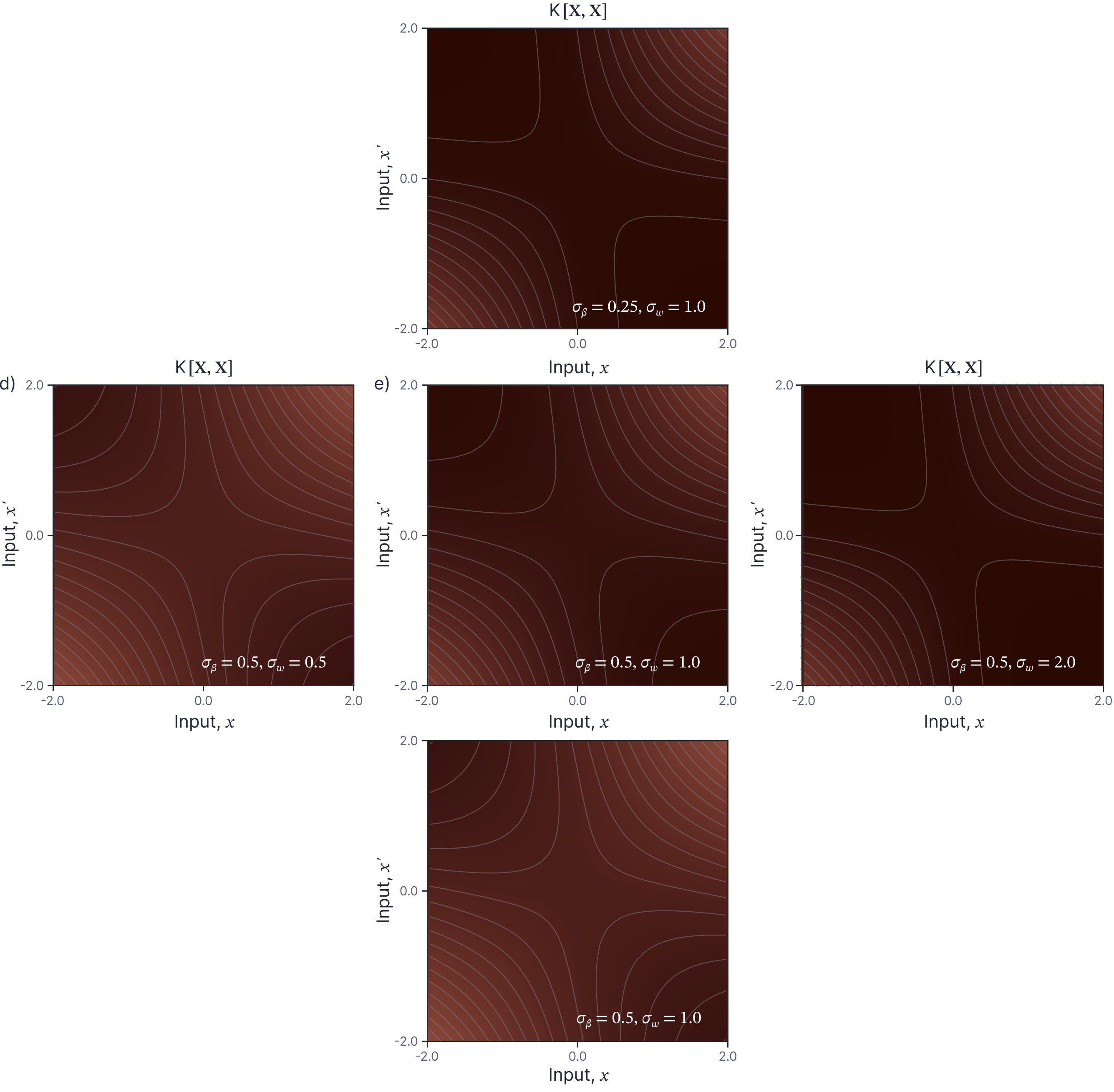
Figure 5. NNGP Kernel. Each panel visualizes the kernel $\mathbf{K}[\mathbf{X},\mathbf{X}]$ for equally spaced points $\mathbf{X}=[x_1, x_2, \ldots x_{I}]$ and for one setting of $\sigma_{\beta}$ and $\sigma_{\omega}$. The horizontal direction represents changes in $\sigma_{\omega}$ and the vertical direction represents changes in $\sigma_{\beta}$.
Figure 6 investigates the kernel with $\sigma_{\beta}=0.5$ and $\sigma_{\omega}=1.0$. The first thing to notice is that the kernel is non-stationary. The kernel function $\mbox{k}[x,x’]$ considered as a function of the input $x$ has a different shape for different values $x’$. This is in contrast to most common kernels such as the RBF kernel where the kernel value depends only on the difference $x-x’$. This explains why random functions drawn from this model have different statistics near the origin (where they change faster) than at larger values (where they become linear, see figure 1c).

Figure 6. NNGP kernel. a) Kernel $\mathbf{K}[\mathbf{X},\mathbf{X}]$ visualized for $\sigma_{\beta}=0.5$ and $\sigma_{\omega}=1.0$. b) Several horizontal cuts through the kernel (i.e., we plot $\mbox{k}[x,x’]$ as a function of $x$ for several different values of $x’$ — depicted by horizontal lines in panel a). It is notable that the kernel is non-stationary; the shape of the kernel depends on the value of $x’$. c) This is in contrast to most common kernels like the RBF kernel (pictured) which depend only on the difference $x-x’$.
Another interesting aspect of the kernel is that the covariance grows as the absolute values of $x$ and $x’$ increase. It might initially seem surprising that larger values co-vary more than smaller ones; some insight into this behaviour is provided if we normalize if we normalize the kernel values as:
\begin{equation}
\tilde{\mbox{k}}[x,x’] = \frac{\mbox{k}[x,x’] }{\sqrt{\mbox{k}[x,x]\mbox{k}[x’,x’]} }.
\tag{20}
\end{equation}
This decomposition reveals that the kernel can be understood as the product of a factor that increases with the magnitude of $x$ and $x’$ and another that assigns more covariance to nearby $x$ and $x’$ (figure 7). In other words, elements $x$ and $x’$ have more individual variance when they are larger, and in addition co-vary more when the distance between them is small.
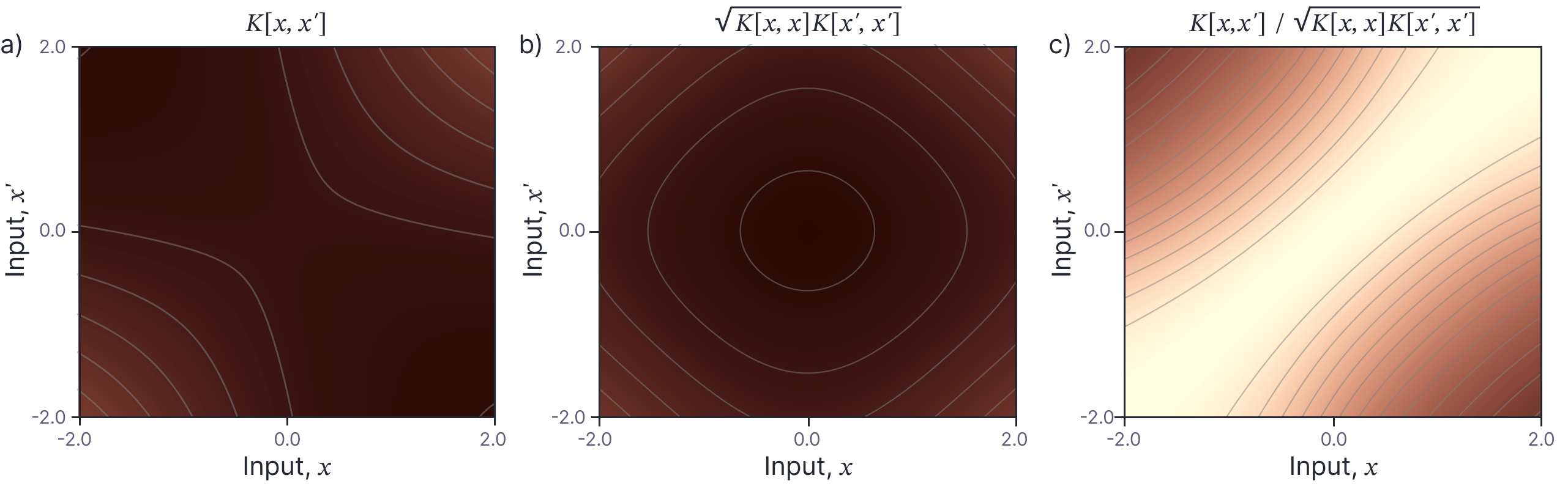
Figure 7. Normalized kernel. a) Neural network kernel for $\sigma_{\beta}=0.5$ and $\sigma_{\omega}=1.0$. This can be understood as being the product of b) a factor that depends on the absolute magnitude of $x$ and $x’$ and c) a factor whereby nearby $x$ and $x’$ values are more highly correlated.
Kernel regression
Now that we have calculated the neural network kernel, we can use it to perform regression, using the methods developed in part V of this series of blogs. We can draw samples from the prior distribution over functions by sampling from:
\begin{equation}
Pr(\mathbf{X}) \sim \mbox{Norm}_{\mathbf{X}}\Bigl[\mathbf{0}, \mathbf{K}\bigl[\mathbf{X},\mathbf{X}\bigr]\Bigr],
\tag{21}
\end{equation}
where $\mathbf{X}=[x_1, x_2, \ldots x_{I}]$ (figure 8a).
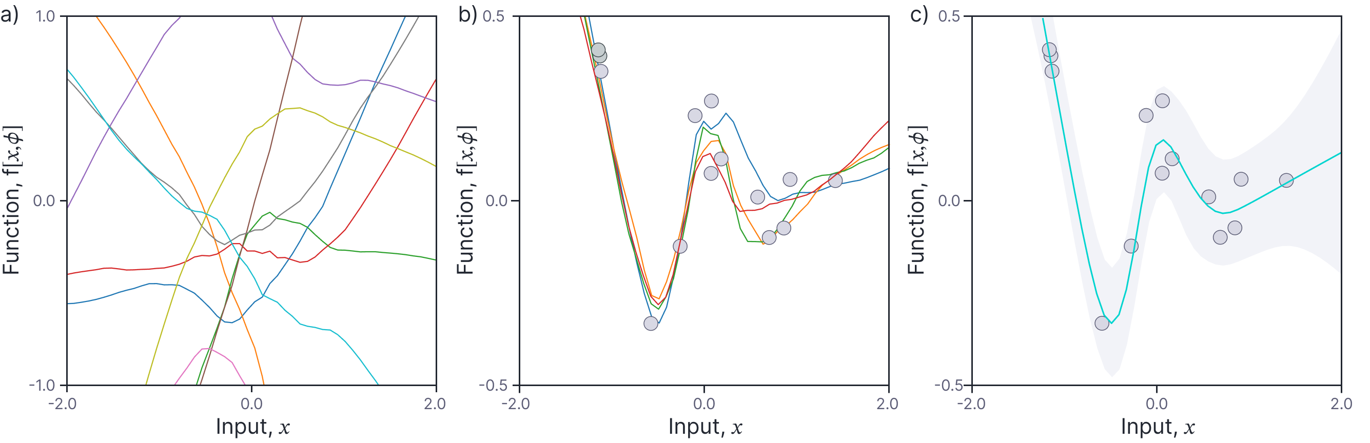
Figure 8. Neural network Gaussian process kernel regression. a) Samples drawn from prior distribution over functions. b) Samples drawn from posterior distribution over functions. c) Mean posterior distribution and marginal uncertainty (gray region represents two standard deviations).
Given a training dataset $\{\mathbf{X},\mathbf{y}\}$ of $I$ examples where $\mathbf{X}=[x_1, x_2, \ldots x_{I}]$ and $\mathbf{y}=[y_1,y_2,\ldots y_I]^T$, we can make predictions $\mathbf{y}^*$ for new examples $\mathbf{X}^{*}$ using:
\begin{eqnarray}\label{eq:NNGP_kernel_regressoin}
Pr(\mathbf{y}^*|\mathbf{X}^*,\mathbf{X},\mathbf{y}) \!\!&\!\!=\!\!&\!\! \mbox{Norm}_{\mathbf{y}^*}\Biggl[\mathbf{K}[\mathbf{X},\mathbf{X}]\biggl(\mathbf{K}[\mathbf{X},\mathbf{X}]+\frac{\sigma^{2}_n}{\sigma^2_p}\mathbf{I}\biggr)^{-1}\mathbf{y},\nonumber \\ &&\hspace{-1.0cm}
\sigma^2_{p}\mathbf{K}[\mathbf{X}^{*},\mathbf{X}^*]\!-\!\sigma^2_{p}\mathbf{K}[\mathbf{X}^*,\mathbf{X}]\biggl(\mathbf{K}[\mathbf{X},\mathbf{X}]+\frac{\sigma^{2}_n}{\sigma^{2}_{p}}\mathbf{I}\biggr)^{-1}\mathbf{K}[\mathbf{X},\mathbf{X}^*]+\sigma^{2}_n\mathbf{I}\Biggr],\nonumber\\
\tag{22}
\end{eqnarray}
where the ratio $\sigma^2_{n}/\sigma^2_{p}$ determines the amount of variation in the training data that can be ascribed to noise. If this is very high, then the model will tend to be smooth and deviate significantly from the training data. If it is very low, then the model will slavishly pass through all of the training data points.
Figure 8b shows a series of samples drawn from the posterior distribution (equation 22). These sample are quite similar close to the data, but diverge in regions that are less constrained. Figure 8c visualizes this in a different way; it shows the mean posterior prediction and the marginal variance for each new input $x$. Again, the variance increases as the points we wish to predict depart significantly from the training data.
Extension to other architectures
It is easy to extend these ideas to build kernels for deep neural networks (Williams et al. 2018, Lee et al. 2018); the covariance of the hidden units in a second layer can be computed by applying the relation in section “Covariance of activations” to the output covariance of the single-layer model; the covariance in the outputs can then be computed by re-applying the relation in section “Covariance of outputs”. Indeed, the same ideas can be applied to different architectures (eg, convolutional networks) and activation functions (e.g. tanh non-linearities).
Empirical performance
Lee et al. (2018) compared the performance of neural network Gaussian processes to that for conventional neural networks (figure 9). For the best choices of hyperparameters for each model, the results are surprisingly similar. It should be noted however that the use of NNGPs is limited by the kernel size. The term $\mathbf{K}[\mathbf{X},\mathbf{X}]$ will be of size $ID\times ID$ for a training data set of $I$ examples, each of which is $D$-dimensional and we must invert a matrix of this size to perform NNGP regression. Although modern approaches allow exact GP inference with a million data points (Wang et al., 2019), this still poses a fundamental limitation on deploying NNGPs.
It is worth noting that the effective performance of NNGPs has been surprising to some researchers (see MacKay 1998); Gaussian processes are usually considered as mere smoothing devices whereas neural networks are seen as learning complex representations of the data. Hence, many researchers feel that something might be lost in extending the networks to infinite width in this way.

Figure 9. NNGP Performance vs. conventional neural networks. Numbers following neural network (NN) are optimal depth, width, and optimization hyperparameters. Numbers following NNGP (GP) are optimal depth, $\sigma^2_{\omega}$, and $\sigma^2_{\beta}$. Adapted from Lee et al. (2018).
Network stability
The analysis of the network covariance inherent to the kernel calculation can also tell us about network stability. If we consider the covariance of two points as the network depth becomes infinite, it may stay stable (in which case the network is trainable), collapse to zero, or diverge to infinity (in which cases the network cannot be trained). These last two scenarios roughly correspond to problems with vanishing and exploding gradients, respectively.
Lee et al. (2018) compared the theoretical network stability (from analysis of the covariance) to the empirical network stability (by experimentation) as a function of the variances $\sigma^2_{\omega}$ and $\sigma^{\beta}$. For ReLU networks, this analysis predicts that we must use He initialization to ensure that the network is stable (figure 10).
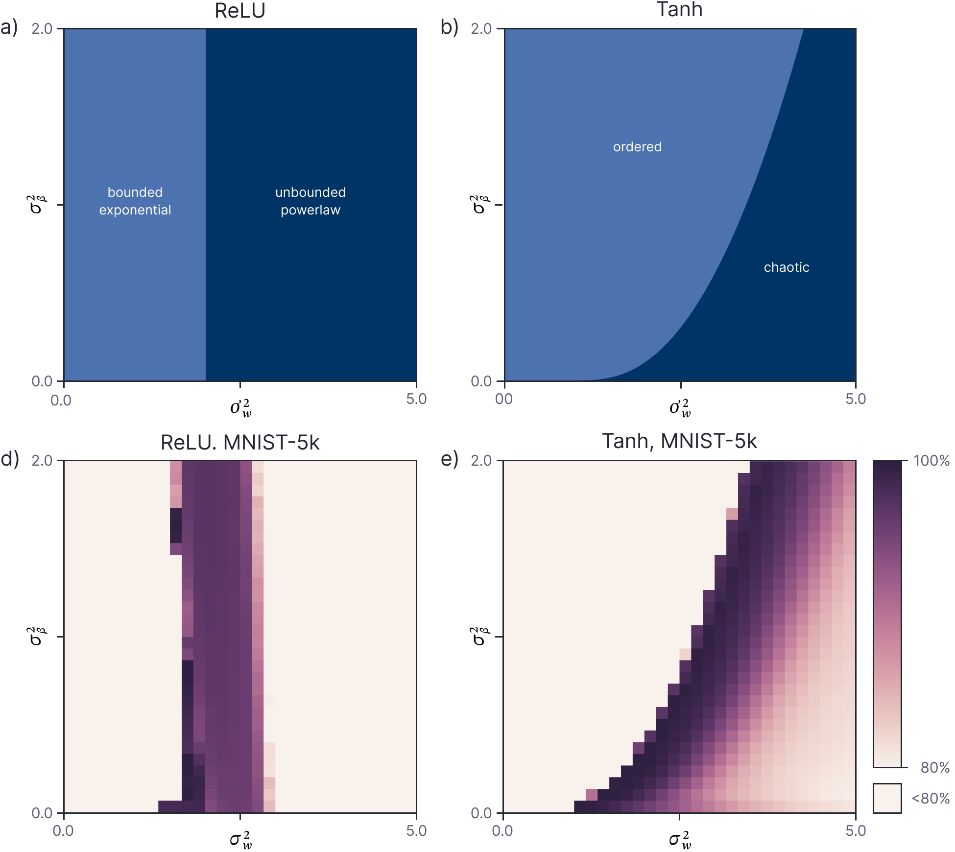
Figure 10. Network stability. a) Theoretical stability analysis for deep ReLU network based on whether distance between two points collapses to zero (left region) or explodes (right region) as a function of $\sigma^2_\beta$ and $\sigma^2_\omega$. There is a critical value of $\sigma^2_\omega=2$ for which the network is stable and this corresponds to He initialization (the typical factor of $1/D$ is eliminated due to the modified network definition). b) The same analysis for tanh activation functions yields a more complex boundary in $\sigma^2_\beta, \sigma^2_\omega$ space. c-d) The empirical accuracy of an NNGP for a 50 layer network with ReLU and tanh non-linearities. Performance is best close to the predicted critical region. Adapted from Lee et al. (2018).
Discussion
This article applied the Bayesian approach (function perspective) to neural networks. We showed that any collection of points passed through an infinitely wide neural network are jointly distributed as a normal distribution; the covariance of this distribution is a captured by the NNGP kernel which can be easily computed. The NNGP is useful both theoretically and practically; the NNGP kernel can provide insights into network stability, and can be used as a supervised learning model for small datasets.
Expected value of ReLU function
The expected value of a normal distribution with mean $\mu$ and variance $\sigma^2$ when passed through a ReLU function can be calculated as:
\begin{eqnarray}
\mathbb{E}[z] &=& \int_{\infty}^{\infty} \mbox{ReLU}[z]\frac{1}{\sqrt{2\pi \sigma^{2}}}\exp\left[\frac{(z-\mu)^{2}}{2\sigma^{2}}\right]dz\nonumber \\
&=& \int_{0}^{\infty} z \frac{1}{\sqrt{2\pi \sigma^{2}}}\exp\left[\frac{-(z-\mu)^{2}}{2\sigma^{2}}\right]dz.
\tag{23}
\end{eqnarray}
Now we make a change of variables $u = (z-\mu)/\sigma$, so $z = \sigma u+\mu$ and $dz = \sigma du$ which yields:
\begin{eqnarray}
\mathbb{E}[z] &=& \int_{-\mu/\sigma}^{\infty} (\sigma u+\mu) \frac{1}{\sqrt{2\pi \sigma^{2}}}\exp\left[\frac{-u^{2}}{2}\right]\cdot \sigma du\nonumber \\
&=& \int_{-\mu/\sigma}^{\infty} (\sigma u+\mu) \frac{1}{\sqrt{2\pi }}\exp\left[\frac{-u^{2}}{2}\right]\cdot du\nonumber \\
&=& \int_{-\mu/\sigma}^{\infty} \sigma u \frac{1}{\sqrt{2\pi}}\exp\left[\frac{-u^{2}}{2}\right]+\mu \frac{1}{\sqrt{2\pi}}\exp\left[\frac{-u^{2}}{2}\right]du\nonumber\\
&=& -\sigma \cdot \mbox{Norm}_x[0,1]\biggr|_{-\mu/\sigma}^\infty+\int_{-\mu/\sigma}^{\infty}\mu \frac{1}{\sqrt{2\pi}}\exp\left[\frac{-u^{2}}{2}\right]du\nonumber\\
&=& \sigma \cdot \mbox{Norm}_{\mu/\sigma}[0,1]+\mu\cdot \int_{-\mu/\sigma}^{\infty}\frac{1}{\sqrt{2\pi }}\exp\left[\frac{-u^{2}}{2}\right]du\nonumber\\
&=& \sigma \cdot \mbox{Norm}_{\mu/\sigma}[0,1]+\mu\cdot \int^{\mu/\sigma}_{-\infty}\frac{1}{\sqrt{2\pi }}\exp\left[\frac{-u^{2}}{2}\right]du\nonumber\\
&=& \sigma \cdot \mbox{Norm}_{\mu/\sigma}[0,1] + \mu\cdot \mbox{cnorm}\left[\frac{\mu}{\sigma}\right],\nonumber
\end{eqnarray}
where the penultimate line follows by the symmetry about zero of the standard normal distribution and $\mbox{cnorm}[x]$ represents the cumulative normal function.