
This blog is the first in a series that describes how ordinary differential equations (ODEs) and stochastic differential equations (SDEs) can be applied to machine learning problems. The series does not assume previous exposure to ODEs and SDEs; a basic knowledge of calculus will suffice to read these articles.
In this article, we give a brief introduction to SDEs and ODEs and discuss the different scenarios in which they are applied to machine learning. In parts II-IV, we introduce ordinary differential equations, how they can be categorized and how they can be solved (either in closed form or numerically). The following articles in the series introduce stochastic differential equations and Itô’s famous lemma.
Armed with this knowledge, subsequent articles in the series will consider how these techniques are used in machine learning. We will see that:
- ODEs can also be used to describe gradient descent with an infinitesimal step size (so-called gradient flow). Similarly, SDEs can be used to describe stochastic gradient descent. These descriptions yield insights about the properties of our optimization algorithms.
- ODEs are combined with deep networks to create neural ODEs in supervised learning and with normalizing flows to create continuous normalizing flows in unsupervised learning. Essentially, these are networks with an infinite number of layers, each of which makes an infinitesimal change to the data representation.
- Both SDEs and ODEs are used in physics-inspired generative models such as diffusion models and Poisson flow models. These are responsible for cutting edge image and video-synthesis models.
- Finally, this relationship can be turned on its head; machine learning can be applied to help solve ODEs and SDEs describing real-world physical processes.
ODEs and SDEs
This section introduces ODEs and SDEs as the limit of discrete sequences of updates to a variable as these updates become smaller but more frequent.
ODEs
Consider an evolving process in a variable $a$:
\begin{equation}
\Delta a= \textrm{m}\bigl[a,t\bigr]\cdot \Delta t.
\tag{1}
\end{equation}
This equation says that a change $\Delta a$ in the variable during a time interval $\Delta t$ can be characterized by a function $\textrm{m}[\bullet,\bullet]$. This function can depend on both the current value of the variable $a$ and the current time $t$. If we knew the value $a$ at time $t=0$, we could run equation 1 repeatedly to find the value of $a$ at times $t=\Delta t, 2\Delta t, \ldots, $ and so on (figure 1a-e).
The related ordinary differential equation (ODE) can be found by considering the limit of this process as the time interval become very small, so $\Delta t \rightarrow dt$ and the corresponding changes in the variable also become small so $\Delta a\rightarrow da$. Here, the notation $d\bullet$ indicates an infinitesimal change.
![ODE example. a-e) The sequence ∆a = (0.5a − 4 sin[t ∗ 10])∆t for time increments ∆t = 0.2,0.1,0.05,0.025,0.0125 with a = 1.0 at time t = 0. f) The associated ODE is formed when the time update ∆t → 0 and the discrete sequence becomes a continuous function.](https://rbcborealis.com/wp-content/uploads/2024/12/DiscreteSequenceODE-v1.png)
Figure 1. ODE example. a-e) The sequence $\Delta a = (0.5a-4 \sin[t*10])\Delta t$ for time increments $\Delta t=0.2, 0.1, 0.05, 0.025, 0.0125$ with $a=1.0$ at time $t=0$. f) The associated ODE is formed when the time update $\Delta t\rightarrow 0$ and the discrete sequence becomes a continuous function.
The evolving process can now be written as:
\begin{equation}
da= \textrm{m}\bigl[a,t\bigr]\cdot dt,
\tag{2}
\end{equation}
or, rearranging:
\begin{equation}
\frac{da}{dt}= \textrm{m}\bigl[a,t\bigr].
\tag{3}
\end{equation}
In general, an ODE is a deterministic relation that describes how the derivatives of a variable $a$ behave. Given a starting value $a_{0}$ we can potentially “solve” the ODE, to find the value of $a$ as a function of time (figure 1f).
SDEs
Now consider adding a small amount of noise $\sqrt{\Delta t}\Delta z$ to the original evolving process:
\begin{equation}
\Delta a= \textrm{m}\bigl[a,t\bigr]\cdot \Delta t + \textrm{s}\bigl[a,t\bigr]\cdot \sqrt{\Delta t}\Delta z,
\tag{4}
\end{equation}
where $\Delta z$ is drawn from a standard normal distribution. The function $\textrm{s}[\bullet,\bullet]$ controls on the contribution of the noise, which can depend on both the current value $a$ and the current time, $t$. The term $\sqrt{\Delta t}$ ensures (non-obviously) that the total amount of noise added in a fixed time interval is the same whatever the step size $\Delta t$.
If we knew the value $a$ at time $t=0$, we could run equation 4 repeatedly to find the value of $a$ at times $t=\Delta t, 2\Delta t,\ldots$. However, this time, the stochastic component $\Delta z$ means that we will not get the same results each time that we ran the sequence.
The related stochastic differential equation (SDE) can be found by considering the limit of this process as the changes in the variable, time interval, and noise become infinitesimal so that $\Delta a\rightarrow da$, $\Delta t \rightarrow dt$ and $\sqrt{\Delta t} \Delta z \rightarrow dw$, where $dw$ is termed a Wiener process:
\begin{equation}
da= \textrm{m}\bigl[a,t\bigr]dt + \textrm{s}\bigl[a,t\bigr]dw,
\tag{5}
\end{equation}
![DE example. a-e) Sequences ∆a = (0.5a − 4 sin[t ∗ 10])∆t + √
0.5 ∆t∆Z for time increments ∆t = 0.2, 0.1, 0.05, 0.025, 0.0125 with a =
1.0 at time t = 0. In each case, the three graphs depict three different
simulations of the sequence; these are different each time because of the
noise element ∆Z. f) The associated SDE is formed when ∆t → 0 and √
∆t∆z → 0.](https://rbcborealis.com/wp-content/uploads/2024/12/DiscreteSequenceSDE-v1.png)
Figure 2. SDE example. a-e) Sequences $\Delta a = (0.5a-4 \sin[t*10])\Delta t + 0.5 \sqrt{\Delta t}\Delta Z$ for time increments $\Delta t=0.2, 0.1, 0.05, 0.025, 0.0125$ with $a=1.0$ at time $t=0$. In each case, the three graphs depict three different simulations of the sequence; these are different each time because of the noise element $\Delta Z$. f) The associated SDE is formed when $\Delta t\rightarrow 0$ and $\sqrt{\Delta t}\Delta z\rightarrow 0$.
This time, we cannot re-arrange the equation to make familiar derivative terms like $da/dt$; we typically leave it just as it is.
In general, an SDE is a stochastic relation that describes how a variable $a$ changes over time. Given a starting distribution $Pr(a|t=0)$ over the value $a$, we can “solve” the SDE to find the distribution $Pr(a|t)$ at other values of $t$.
ODEs and SDEs in machine learning
Let’s now consider how ODEs and SDEs relate to machine learning. To do this, we identify situations with deterministic evolving sequences (suited to ODEs) and noisy evolving sequences (suited to SDEs).
Gradient descent
In gradient descent, the parameters $\boldsymbol\phi$ of a model evolve according to the relation:
\begin{equation}
\boldsymbol\phi_{t+1} = \boldsymbol\phi_{t} – \alpha \sum_{i=1}^I\frac{\partial l[\mathbf{x}_i,\boldsymbol\phi_t]}{\partial \boldsymbol\phi},
\tag{6}
\end{equation}
where $\alpha \in \mathbb{R}^+$ is the learning rate and $l[\mathbf{x}_{i}, \boldsymbol\phi]$ is the loss term associated with the $i^{th}$ of $I$ training examples (figure 3). This can be re-arranged to:
\begin{equation}
\boldsymbol\phi_{t+1} – \boldsymbol\phi_{t} = – \alpha \sum_{i=1}^I\frac{\partial l[\mathbf{x}_i,\boldsymbol\phi_t]}{\partial \boldsymbol\phi},
\tag{7}
\end{equation}
and writing $\Delta\boldsymbol\phi_{t} = \boldsymbol\phi_{t+1} – \boldsymbol\phi_{t}$, we get:
\begin{equation}
\Delta\boldsymbol\phi_t = – \alpha \sum_{i=1}^I\frac{\partial l[\mathbf{x}_i,\boldsymbol\phi_t]}{\partial \boldsymbol\phi},
\tag{8}
\end{equation}
This is a deterministic process that is a special case of equation 1 where the variable $a$ has been replaced by the parameters $\boldsymbol\phi$ and the change in time by $\Delta t=1$. The function $m[\bullet, \bullet]$ is given by the negative learning rate times the sum of the gradients at position $\boldsymbol\phi_{t}$. In this case, this function does not depend directly on the value of $t$ itself.

Figure 3. Gradient descent and stochastic gradient descent. a) In gradient descent the parameters evolve according to a deterministic rule. If we make the learning rate infinitesimal, this evolution can be described by an ordinary differential equation. b) In stochastic gradient descent, the parameters evolve based on a stochastic rule. If we make the learning rate infinitesimal, this evolution can be described by a stochastic differential equation. Adapted from $\href{https://udlbook.com}{\color{blue}Prince (2023)}$.
The equivalent ODE can be found by taking the limit of this process as $\Delta \boldsymbol\phi\rightarrow d\boldsymbol\phi$ and $\Delta t \rightarrow dt$, which gives the gradient flow equation:
\begin{equation}
d\boldsymbol\phi_t = – \alpha \sum_{i=1}^I\frac{\partial l[\mathbf{x}_i,\boldsymbol\phi_t]}{\partial \boldsymbol\phi}dt,
\tag{9}
\end{equation}
or, rearranging:
\begin{equation}
\frac{d\boldsymbol\phi_t}{dt} = – \alpha \sum_{i=1}^I\frac{\partial l[\mathbf{x}_i,\boldsymbol\phi_t]}{\partial \boldsymbol\phi}.
\tag{10}
\end{equation}
The gradient flow equation will provide a lens to understand how learning in machine learning models occurs in an idealized case.
Stochastic gradient descent
Stochastic gradient descent can similarly be written as:
\begin{equation}
\Delta\boldsymbol\phi_t = – \alpha \sum_{i\in \mathcal{B}_{t}}\frac{\partial l[\mathbf{x}_i,\boldsymbol\phi_t]}{\partial \boldsymbol\phi},
\tag{11}
\end{equation}
where $\mathcal{B}_t$ is the set of training data indices in the batch at step $t$. We can approximate this by considering that there is an independent fixed probability that each example will be in any given batch. Denoting inclusion of the $i^{th}$ training example in the batch at time $t$ by the random variable $b_{i,t}\in\{0,1\}$, we can equivalently write:
\begin{equation}
\Delta\boldsymbol\phi_t = – \alpha \sum_{i=1}^I b_{it}\frac{\partial l[\mathbf{x}_i,\boldsymbol\phi_t]}{\partial \boldsymbol\phi}.
\tag{12}
\end{equation}
This right-hand side is now expressed as the sum of independent and identically distributed variables and so by the central limit theorem, we expect the udpate to be normally distributed with some mean $\boldsymbol\mu[\boldsymbol\phi, t]$ and some standard deviation $\boldsymbol\sigma[\boldsymbol\phi, t]$:
\begin{equation}
\Delta\boldsymbol\phi_t = – \alpha \boldsymbol\mu[\boldsymbol\phi, t] – \alpha \boldsymbol\sigma[\boldsymbol\phi, t] \Delta z
\tag{13}
\end{equation}
where $\Delta z$ is noise drawn from a standard normal distribution. This is clearly a special case of the general stochastic evolving process in equation 4, where again $\Delta t=1$.
It follows that there is an associated SDE that describes how stochastic gradient descent would work in the infinitesimal limit:
\begin{equation}
d \boldsymbol\phi_t = – \alpha \boldsymbol\mu[\boldsymbol\phi, t]dt – \alpha \boldsymbol\sigma[\boldsymbol\phi, t] dw.
\tag{14}
\end{equation}
This equation will provide insights into how quantities such as the learning rate and batch size affect the training process. Part IV of this blog will investigate the implications of using ODEs and SDEs to describe parameter optimization.
Residual networks
The simplest deep networks process data sequentially; each layer receives the previous layer’s output and passes the result to the next (figure 4). For example, a three-layer network is defined by:
\begin{eqnarray}\label{eq:residual_sequential}
\textbf{ h}_1 &=& \textbf{ f}_{1}[\mathbf{x},
\boldsymbol\phi_{1}]\nonumber \\
\textbf{ h}_2 &=& \textbf{ f}_{2}[\mathbf{h}_{1},\boldsymbol\phi_{2}]\nonumber \\
\textbf{ h}_3 &=& \textbf{ f}_{3}[\mathbf{h}_{2},\boldsymbol\phi_{3}]\nonumber \\
\mathbf{y} &=& \textbf{ f}_{4}[\mathbf{h}_{3},\boldsymbol\phi_{4}],
\tag{15}
\end{eqnarray}
where $\mathbf{h}_{1}$, $\mathbf{h}_{2}$, and $\mathbf{h}_{3}$ denote the intermediate hidden layers, $\mathbf{x}$ is the network input, $\mathbf{y}$ is the output, and the functions $\textbf{ f}_{k}[\bullet,\boldsymbol\phi_{k}]$ perform the processing. The representation evolves deterministically as it moves through the network just as in equation 1, so the network could potentially be described by an ODE in the infinitesimal regime.
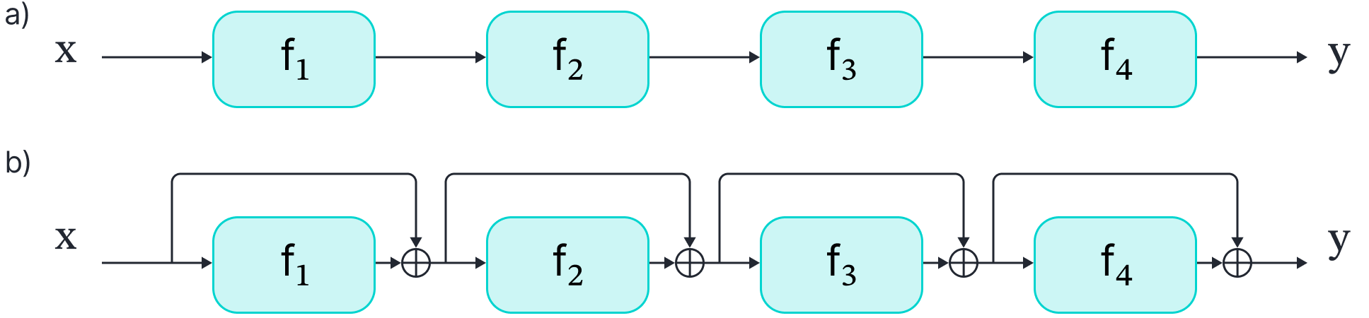
Figure 4. Residual networks. a) A standard network process the input data sequentially through a number of layers. b) A residual network computes a new function of the data and adds it back to the current representation at each stage. As these changes become infinitesimal, this process can be represented by an ordinary differential equation. Adapted from $\href{https://udlbook.com}{\color{blue}Prince (2023)}$.
However, it is more natural to work with residual networks. These contain branches in the computational path known as residual or skip connections. At each stage, the input to each network layer $\textbf{ f}[\bullet]$ is added back to the output (figure 4b). By analogy to equation 15, the residual network is defined as:
\begin{eqnarray}
\mathbf{h}_{1} &=& \mathbf{x} + \textbf{ f}_{1}[\mathbf{x},\boldsymbol\phi_{1}]\nonumber \\
\mathbf{h}_{2} &=& \mathbf{h}_{1} + \textbf{ f}_{2}[\mathbf{h}_{1},\boldsymbol\phi_{2}]\nonumber \\
\mathbf{h}_3 &=& \mathbf{h}_{2} + \textbf{ f}_{3}[\mathbf{h}_{2},\boldsymbol\phi_{3}]\nonumber \\
\mathbf{y} &=& \mathbf{h}_{3} + \textbf{ f}_{4}[\mathbf{h}_{3}, \boldsymbol\phi_{4}],
\tag{16}
\end{eqnarray}
where the first term on the right-hand side of each line is the residual connection. Each function $\textbf{ f}_{k}$ learns an additive change to the current representation with the general relation:
\begin{equation}
\mathbf{h}_{t+1} = \mathbf{h}_{t} + \textbf{ f}_t\bigl[\mathbf{h}_{t},\boldsymbol\phi_{t+1}\bigr]\cdot \Delta t
\tag{17}
\end{equation}
where $\Delta t=1$ for a standard residual network.
Now, we re-arrange equation 17 as:
\begin{equation}
\mathbf{h}_{t+1}- \mathbf{h}_{t}=\textbf{ f}\bigl[\mathbf{h}_{t},\boldsymbol\phi_{t+1}\bigr]\cdot\Delta t
\tag{18}
\end{equation}
or
\begin{equation}
\Delta \mathbf{h} =\textbf{ f}\bigl[\mathbf{h},\boldsymbol\phi_{t+1}\bigr]\cdot \Delta t.
\tag{19}
\end{equation}
Now consider adding more and more layers, each of which makes a smaller and smaller change. Taking the infinitesimal limit and moving the $\Delta t$ term to the left and side, we get:
\begin{equation}
\frac{d \mathbf{h}}{dt} =\textbf{ f}\bigl[\mathbf{h},\boldsymbol\phi, t\bigr],
\tag{20}
\end{equation}
where the network layers are now instantiated by using $t$ as an explicit input to the model equation. This is known as a neural ODE.
Other types of network can also be considered in the infinitesimal limit. For example, normalizing flows model probability density by sequentially warping a base distribution (typically a normal distribution) to the desired distribution. As for residual networks, we can consider the limit of this process as the number of layers becomes infinite, but their contribution becomes smaller. This yields continuous normalizing flows. Both neural ODEs and continuous normal flows will be discussed in part V of this series of articles.
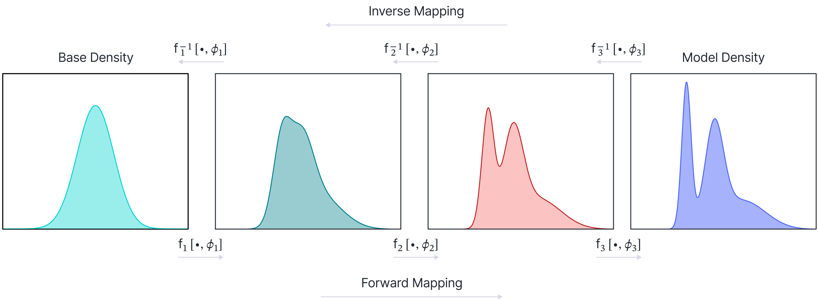
Figure 5. Normalizing flows. A base density is gradually transformed by a sequence of network layers to a probability distribution that matches the observed data. To sample from this model, we draw from the base density and then transform the result through the network (forward mapping). To evaluate the probability for a point, we transform the point backwards through the network (inverse mapping). The final probability depends both on the warping process and the base density of the transformed point. Consider increasing the number of steps in this process but changing the density by a smaller amount at each step. In the limit of infinitesimal changes, the model can be described by an ODE and is termed a $\textit{continuous}$ $\textit{normalizing flow}$
Diffusion models
Diffusion models are generative models that can be used to synthesize new images. They consist of an encoder and a decoder. In the encoder, noise is gradually added to the image:
\begin{eqnarray}
\mathbf{h}_{1} &=& \sqrt{1-\beta_{1}}\cdot \mathbf{x} + \sqrt{\beta_{1}}\cdot \boldsymbol\epsilon_{1} \\
\mathbf{h}_{t} &=& \sqrt{1-\beta_{t}}\cdot \mathbf{h}_{t-1} + \sqrt{\beta_{t}}\cdot \boldsymbol\epsilon_{t} \quad\quad\quad \forall\hspace{1mm} t \in2,\ldots, T,\nonumber
\tag{21}
\end{eqnarray}
where $\mathbf{x}$ is the original image, $\mathbf{h}_{t}$ is the noisy image at step $t$, $\epsilon_{t}$ is random noise drawn from a standard normal distribution and the terms $\beta_t\in[0,1]$ determine the amount of noise that is added at each step. The decoder consists of a series of neural networks that attempt to reverse this process (figure 6). After training, we can generate an image containing random noise and use the decoder to turn it into a realistic image.
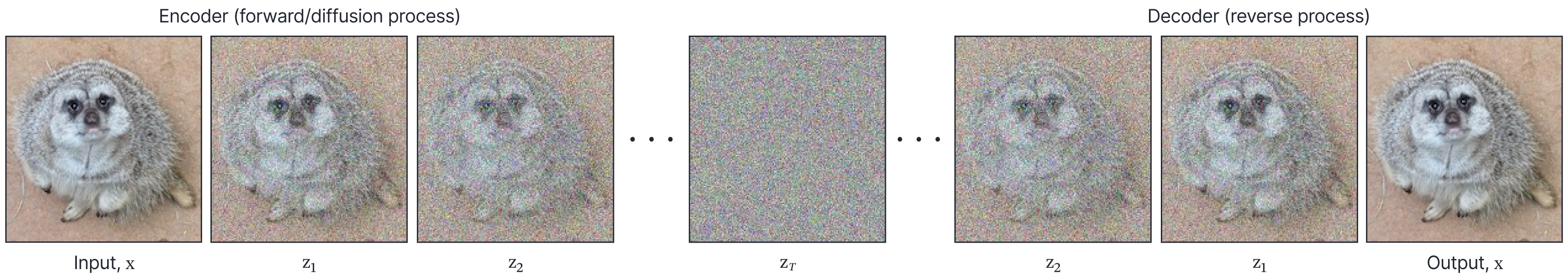
Figure 6. Diffusion models. In the encoder, the input image is gradually transformed to pure noise, by repeatedly reducing the amount of signal and adding a small noise component. The decoder is a machine learning model that reverses this process. In the infinitesimal limit, both the encoder and decoder can be described by an SDE.
The general encoder step can be re-written as
\begin{equation}
\mathbf{h}_{t}-\mathbf{h}_{t-1} = (\sqrt{1-\beta_{t}}-1)\cdot \mathbf{h}_{t-1} + \sqrt{\beta_{t}}\cdot \boldsymbol\epsilon_{t}
\tag{22}
\end{equation}
or alternatively:
\begin{equation}
\Delta \mathbf{h}_{t} = (\sqrt{1-\beta_{t}}-1)\cdot \mathbf{h}_{t-1} + \sqrt{\beta_{t}} \cdot \Delta\mathbf{z}
\tag{23}
\end{equation}
Taking the infinitesimal limit, we see that this is a special case of a more general stochastic differential equation known as a diffusion model:
\begin{equation}
d\mathbf{h} = \textbf{m}[\mathbf{h},t]dt + s[t]d\mathbf{w},
\tag{24}
\end{equation}
The reverse process (in which we start with random noise and transform it to make an image) can also be described by an SDE and it is the terms of this reverse SDE that we learn when we train a diffusion model.
In fact, diffusion models are part of a larger class of physics-based generative models which use ODEs and SDEs to describe the mapping between an image and a random noise sample. These will be discussed in detail in part VI of this series.
Physics-informed machine learning
The previous applications have all discussed how ODEs and SDEs can be applied to understand machine learning algorithms or build new machine learning models. However, machine learning can also be used to help solve problems in the real world that are governed by ODEs and SDEs. For example, machine learning can be used to speed up simulation of known physical processes, or even to discover new physical processes. Such physics-informed machine learning applications are discussed in part VII of this series.
Conclusion
This article has identified a number of places where ordinary differential equation and stochastic differential equations are related to deep learning models. Part II and part III of this series will investigate the properties of ODEs and SDEs in general.