
In part V of this series on ODEs and SDEs in machine learning, we introduced stochastic processes. We saw that an SDE is an implicit representation of a stochastic process and “solving” the SDE involves recovering this stochastic process (or at least information about its moments). We introduced the simple SDE $dx=dw$ and defined its solution to be the Wiener process $W_t$.
In part VI of the series (this article) we consider how to solve more complex SDEs in closed form. We argue that when both the diffusion and drift term of the SDE depend only on the independent variable $t,$ the solution is straightforward; we simply integrate the equation. This raises the question of how to integrate the diffusion (noise) term.
To this end, we introduce the stochastic integral. We see that this has many properties in common with the standard Riemann integral but others that are quite different. The solution to a stochastic integral is a random variable, and we derive expressions for the mean and variance of this variable.
Restricting SDEs to integrable form
Our goal is to solve stochastic differential equations which have the general form:
\begin{equation}\label{eq:ode6_general_sde}
dx = \mbox{m}[x,t] dt + \mbox{s}[x,t] dw,
\tag{1}
\end{equation}
where $x$ is the dependent variable and $t$ is the independent variable (usually representing time). The term $dx$ represents an infinitesimal change in the dependent variable, $dt$ represents an infinitesimal change in time, and $dw$ represents an infinitesimal noise shock. The drift term $\mbox{m}[x,t]$ and the diffusion term $\mbox{s}[x,t]$ control the magnitude of the deterministic and stochastic changes to the variable, respectively.
This general form of SDE is challenging to solve since the drift and diffusion terms both depend on the dependent variable $x$. This value is perturbed randomly by the diffusion term at each infinitesimal time step, and this in turn affects subsequent drift and diffusion contributions; the future trajectory is influenced in a complex and uncertain way by the noise at the current time (figure 1).
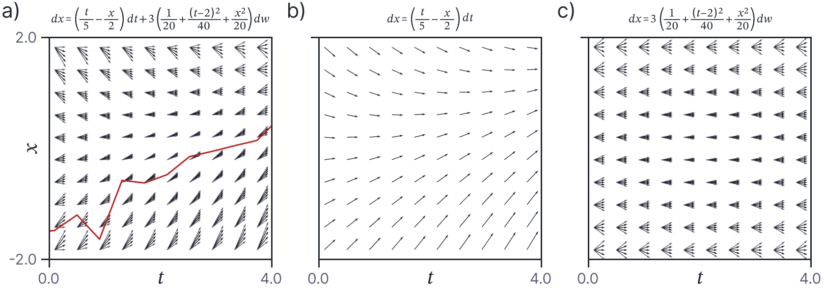
Figure 1. General SDE of the form in equation 1. a) The full SDE. Orange curve represents one (coarsely sampled) path through the SDE. b) The drift (deterministic) term. c) The diffusion (stochastic) term. Unfortunately, both the drift and diffusion terms depend on the variable $x$ (i.e., the columns of the fields in panels b and c are not constant), so the noise from the diffusion term affects the future trajectory in complex and indirect ways. This makes the SDE difficult to solve.
Things are much simpler if we restrict the forms of the drift and diffusion terms. In particular, we’ll initially assume that they depend only on the independent variable $t$ and not on the dependent variable $x$:
\begin{equation}\label{eq:ode6_restricted_sde}
dx = \mbox{m}[t] dt + \mbox{s}[t] dw.
\tag{2}
\end{equation}
Now, the random perturbations to $x$ made by the noise do not modify the future effect of either the deterministic drift term or the stochastic diffusion term since both depend only on $t$ (figure 2); the increments at each time step are now independent. To solve this SDE using initial condition $x=x_0$ at time $t=0$, we simply integrate both sides:
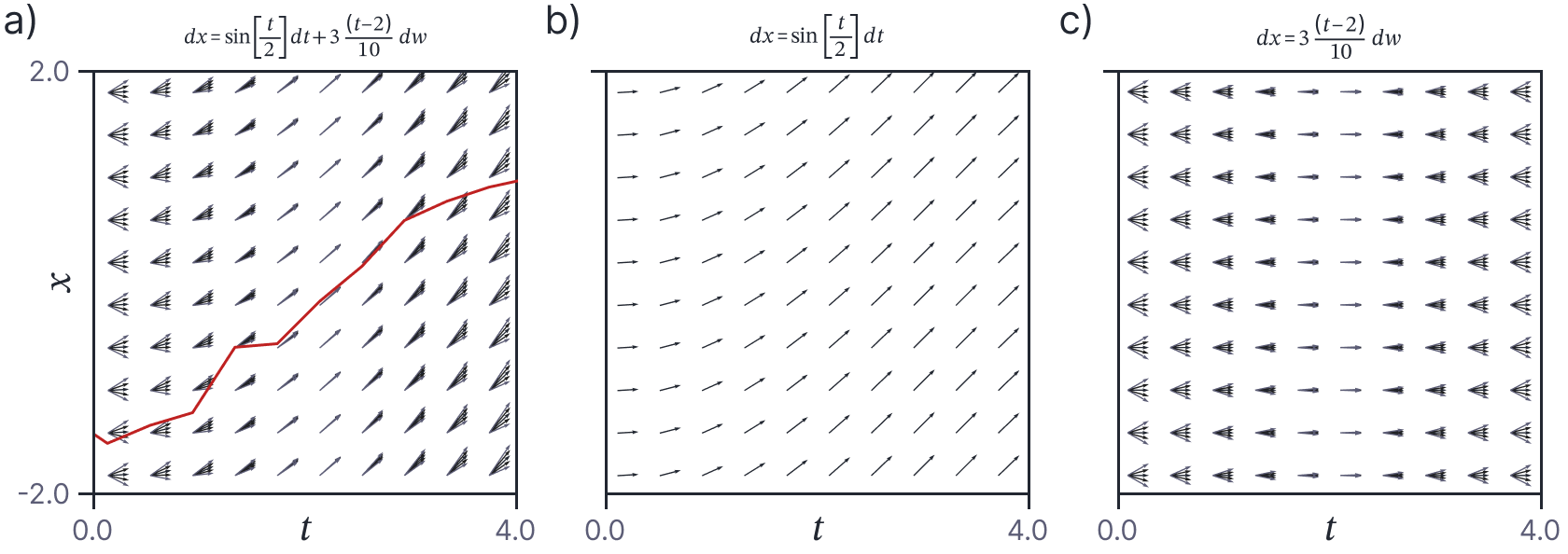
Figure 2. Restricted SDE of the form in equation 2. a) The full SDE. Orange curve represents one (coarsely sampled) path through the SDE. b) The drift (deterministic) term. c) The diffusion (stochastic) term. For this SDE, both the drift and diffusion terms depend on $t$ alone (i.e, the columns of the panels are constant). Hence, historical changes to the dependent variable $x$ do not affect the distribution of changes at the current time, and we can solve this SDE, by simply integrating the changes over time.
\begin{equation}\label{eq:ode6_general_form}
x_t = x_0+ \int_0^t \mbox{m}[\tau] d\tau + \int_0^t \mbox{s}[\tau] dw_\tau.
\tag{3}
\end{equation}
The first integral on the right-hand side is a standard Riemann integral. However, the second integral is stochastic integral. This stochastic integral does not behave in the same way as the standard Riemann integral that you are used to; it obeys the rules of stochastic calculus.
Riemann integral
Before we tackle the stochastic integral, let’s review the definition of the Riemann integral (i.e., the first integral on the right hand side of equation 3). We start by dividing the time interval $t$ into $N$ segments of width $t/N$, starting at $t_{0}, t_{1},\ldots, t_{N-1}$. We then define the Riemann sum as:
\begin{equation}
I_N[t] = \sum_{n=0}^{N-1}\mbox{m}[t_n] \bigl(t_{n+1} – t_n\bigr).
\tag{4}
\end{equation}
This has a clear geometric interpretation; we sum together the area of rectangular regions each of which has width $t_{n+1} – t_n=t/N$. The heights of the regions are given the points $\textrm{m}[t_0], \textrm{m}[t_1],\ldots \textrm{m}[t_{N-1}]$ at the left boundary of the interval. The Riemann integral $I[t]$ is the limit of the Riemann sum as the number of intervals $N$ increases and their width $t/N$ decreases commensurately (figure 3):
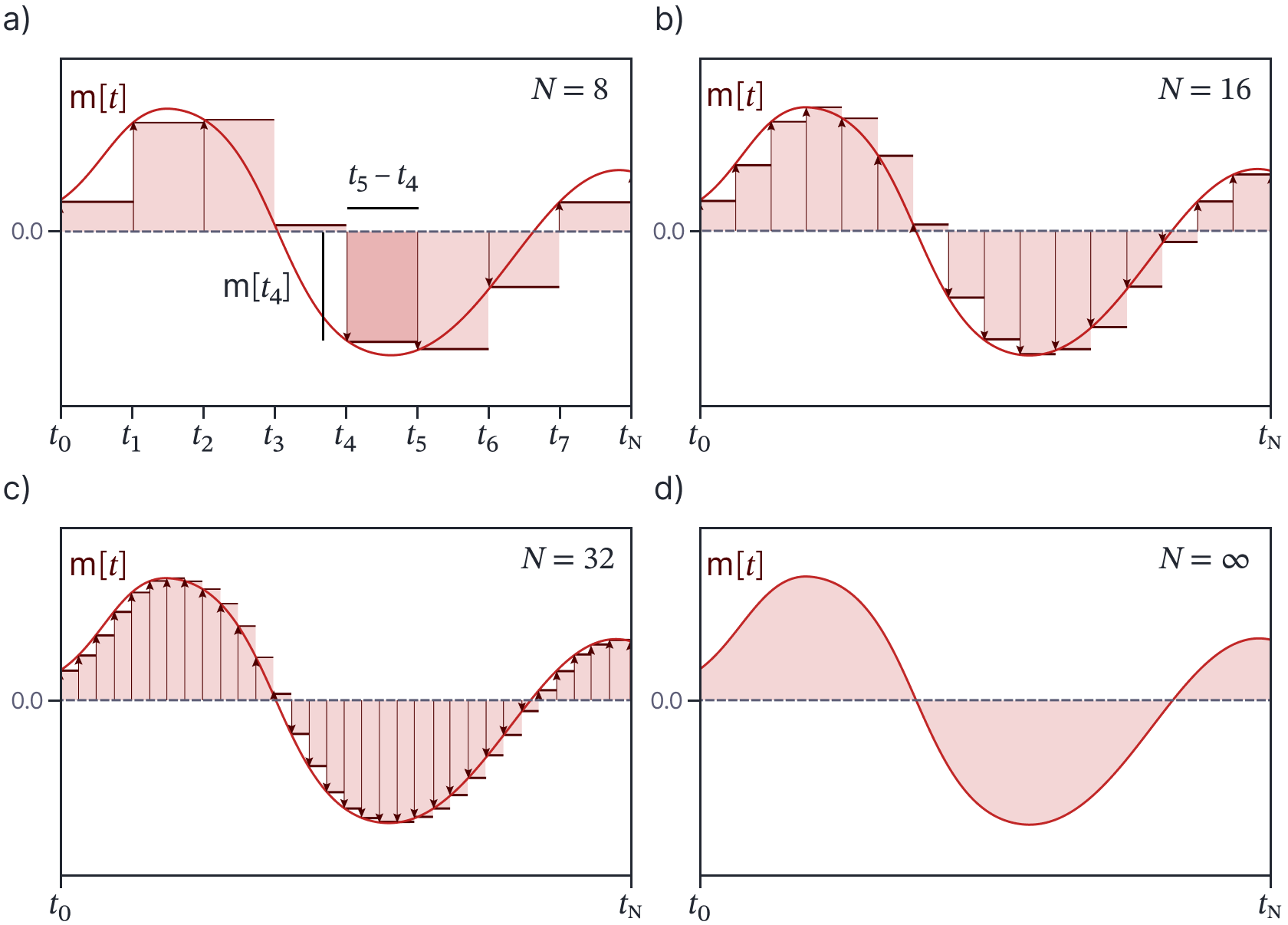
Figure 3. The Riemann (standard) integral. a) The integral aims to compute the (signed) total area under the orange curve of interest $\mbox{m}[t]$ in some region. We approximate this area by dividing the variable $t\in[0,t]$ (horizontal axis) into $N=8$ regions $\{t_1,t_2,\ldots, t_N\}$. We then compute the sum of the signed areas of the eight rectangular regions. The width of the $n^{th}$ region is given by $t_{n+1}-t_{n}=t/n$, and the height is given by the height $\mbox{m}[t_{n}]$ of the curve at the left of the region. b-c) This approximation increases in accuracy as the number of regions increases. d) The Riemann integral is defined as the limit of this sequence where we have an infinite number of regions of infinitesimal width.
\begin{eqnarray}\label{eq:ode6_riemann_integral}
I[t] = \int_0^t \mbox{m}[\tau] d\tau &=& \lim_{N\rightarrow\infty} I_{N}[t] \nonumber \\
&=& \lim_{N\rightarrow\infty} \sum_{n=0}^{N-1}\mbox{m}[t_n] \bigl(t_{n+1} – t_n\bigr).
\tag{5}
\end{eqnarray}
Stochastic integrals
Now we turn to the stochastic integral (i.e., the second integral on the right hand side of equation 3). This a special case of the more general stochastic integral:
\begin{equation}
I[t] = \int_0^t \mbox{s}\bigl[W_\tau, \tau\bigr] dw_\tau,
\tag{6}
\end{equation}
where the integrand $\mbox{s}[W_\tau, \tau]$ is also stochastic because it depends on a Wiener process $W_{\tau}$. This is known as an Itô integral and the restriction to the case where the integrand $\mbox{s}[t]$ is deterministic is known as a Wiener integral. We will work with the more general formulation for now.
The corresponding Riemann sum is defined as:
\begin{equation}
I_N[t, W_t] = \sum_{n=0}^{N-1} \textrm{s}\bigl[W_{t_{n}}, t_n\bigr]\bigl(W_{t_{n+1}} – W_{t_n}\bigr).
\tag{7}
\end{equation}
Once more, we now consider the case where the number of intervals $N$ increases to infinity and the width of the intervals decreases to zero. Itô showed that there exists a random variable $I[t]$ that is the L2 limit:
\begin{equation}
\mathbb{E}\Bigl[\bigl(I_{t_N} – I[t]\bigr)^2\Bigr]\rightarrow 0 \quad\quad \textrm{as } N\rightarrow\infty,
\tag{8}
\end{equation}
and called this limit the stochastic integral:
\begin{eqnarray}\label{eq:ode6_stochastic_integral}
I[t] = \int_0^t \mbox{s}\bigl[W_\tau,\tau\bigr] dw_\tau &=& \lim_{N\rightarrow\infty} I_{N}[W_t, t] \nonumber \\
&=& \lim_{N\rightarrow\infty} \sum_{n=0}^{N-1}\mbox{s}\bigl[W_{t_n}, t_n\bigr] \bigl(W_{t_{n+1}} – W_{t_n}\bigr).
\tag{9}
\end{eqnarray}
This is now commonly referred to as the Itô integral.
Wiener integral intuition
The mathematical exposition of the previous section provides little intuition into what exacly the stochastic integral represents. To gain some insight, let’s first consider the simpler Wiener integral (where the integrand is deterministic):
\begin{equation}\label{eq:ode6_wiener_integral_limit}
I[t] = \int_0^t \mbox{s}\bigl[\tau\bigr] dw_\tau
= \lim_{N\rightarrow\infty} \sum_{n=0}^{N-1}\mbox{s}\bigl[t_n\bigr] \bigl(W_{t_{n+1}} – W_{t_n}\bigr).
\tag{10}
\end{equation}
We know from the properties of the Wiener process that $W_{t_{n+1}} – W_{t_n}$ is the same as $W_{t_{n+1}-t_{n}}= W_{t/N}$ which is distributed as $\mbox{Norm}[0, t/N]$. Hence, the summation term in equation 10 combines $N$ random variables from times $t_{0}\ldots t_{N-1}$ which are randomly distributed with mean zero and standard deviation $\textrm{s}[t_n]\cdot \sqrt{t/N}$ (figure 4). The sum of independently drawn mean-zero normally distributed variables is itself a mean-zero normally distributed variable. It follows that (i) the result of the summation is a random variable and (ii) this random variable is normally distributed with mean zero.
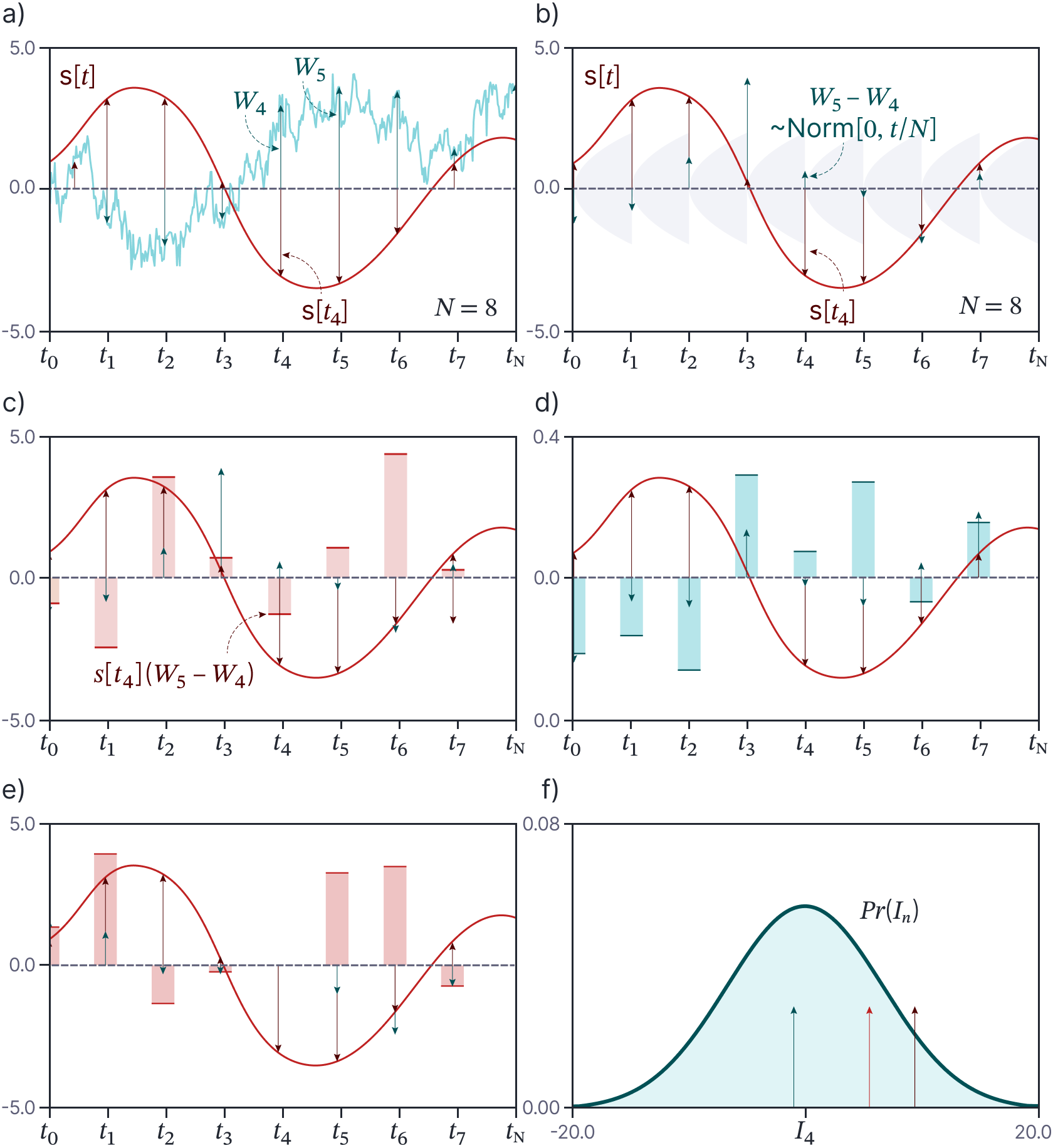
Figure 4. Wiener integral. a) Consider the function $\textrm{s}[t]$ that we wish to integrate (orange curve) and a Wiener process $W_{t}$ defined on the same interval (cyan curve). We can approximate the integral by dividing the original interval $t$ into $N=8$ regions. Each element of the sum $\mbox{s}\bigl[t_n\bigr] (W_{t_{n+1}} – W_{t_n})$ is computed from (i) the height of the curve $\mbox{s}[t_n]$ at the leftmost point in the region (orange arrows), (ii) the value of the Wiener process $W_{t_{n}}$ at the leftmost point in the region (green arrows) and (iii) the value of the Wiener process $W_{t_{n+1}}$ at the rightmost point in the region (subsequent green arrows). b) From the properties of the Wiener process, we know that $W_{t_{n+1}} – W_{t_n}\sim \textrm{Norm}[0,t/N]$ and so we can equivalently think of each element of the sum as consisting of $\mbox{s}[t_n]$ (brown arrows) and a noise term $W_{t/N}$ drawn from $\textrm{Norm}[0,t/N]$ (green arrows). c) To approximate the integral, we pointwise multiply these two sets of quantities to yield values $\mbox{s}_{n}W_{t/N}$ (heights of shaded areas) and sum the results. d-e) Each time we do this, we get a different answer (due to the randomness inherent in the Wiener process). f) It follows that the Itô integral for a deterministic function $\mbox{s}[t]$ is a normally distributed random variable (arrows represent the draws from this variable computed in panels c-e).
Figure 5 shows how the summations change as we increase the number of regions $N$. When we double the number of regions, the number of terms in the summation increases, but the standard deviation $\textrm{s}[t_n]\cdot \sqrt{t/N}$ of each term decreases to compensate for the additional terms. The Wiener integral is the limit of this process as the number of terms becomes infinite.
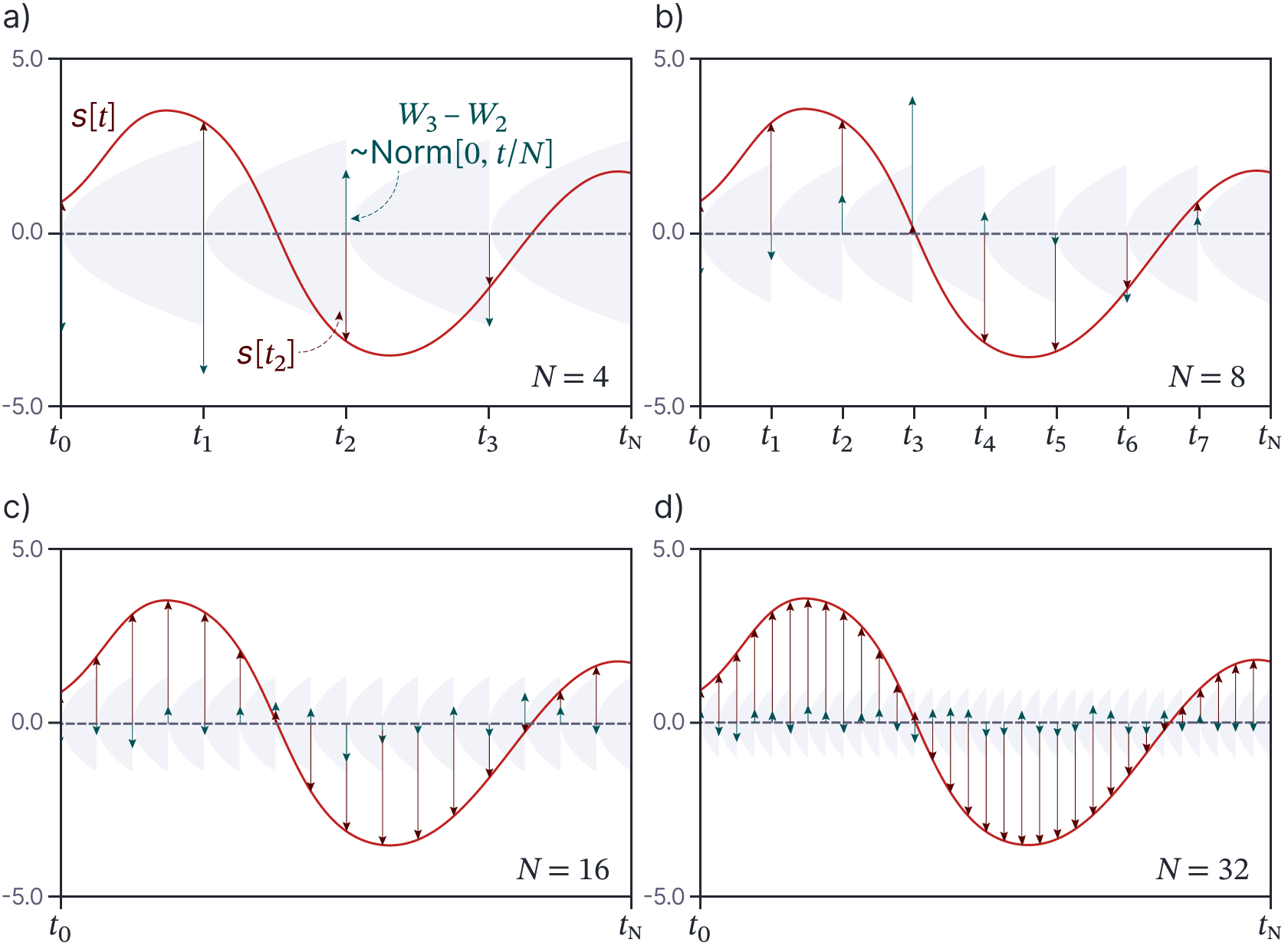
Figure 5. Limit of approximation to Wiener integral. Just as for the Riemann integral, the Itô integral is defined as the limit of a series of approximations which divide the interval $[0,t]$ into an increasingly large number of ever-smaller intervals. a-d) The approximation with $N=4,8,16$, and $32$ intervals, respectively. As the intervals become smaller, the variance of the Wiener process $W_{t/N} = W_{t_{n+1}}\! -\! W_{t_n}$ becomes correspondingly smaller to compensate for the increased number of terms in the sum.
Itô integral intuition
Now consider the full Itô integral:
\begin{equation}\label{eq:ode6_ito_integral_limit}
I[t] = \int_0^t \mbox{s}\bigl[W_\tau, \tau\bigr] dw_\tau
= \lim_{N\rightarrow\infty} \sum_{n=0}^{N-1}\mbox{s}\bigl[W_{\tau}, t_n\bigr] \bigl(W_{t_{n+1}} – W_{t_n}\bigr).
\tag{11}
\end{equation}
The $n^{th}$ term in the sum on the right-hand side takes three contributions. First it uses the height $\mbox{s}[W_{t_n},t_n]$ of the stochastic integrand at the leftmost side point in the region. Second it uses the value $W_{t_n}$ of the Wiener process at the leftmost point in the region. Finally, it uses the value $W_{t_{n+1}}$ of the Wiener process at the rightmost point in the region.
Once more the sum is a random variable. This time we have a sum of products of Gaussians. Moreover the three terms $\mbox{s}[W_{t_n},t_n]$, $W_{t_n}$ and $W_{t_{n+1}}$ are computed from the same Wiener process. We will shortly see that the resulting random variable has mean zero but is typically not normally distributed; figure 6 shows the example $\mbox{s}[W_t,t]=2W_{t}$ for which the random variable representing the integral is a scaled and shifted $\chi$-squared distribution.
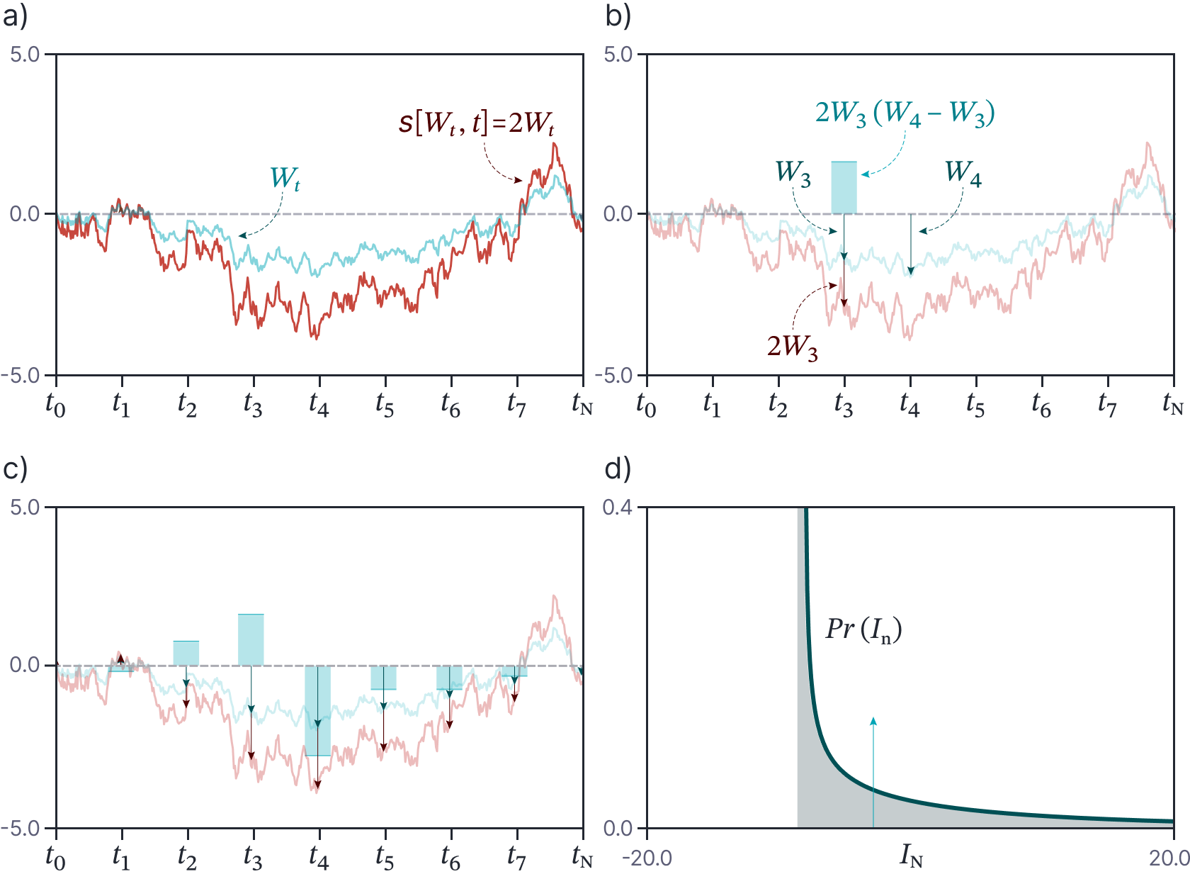
Figure 6. Itô (stochastic) integral for $\mbox{s}[W_t,t]=2W_t$. a) The integral is approximated from a Wiener process $W_t$ and the function $\mbox{s}[W_t,t]$. b) To compute the fourth term $S_{3}[W_3,t_3](W_4-W_3)$ in the sum, we use the value of the integrand $\mbox{s}[W_3,3]=2W_3$ (orange arrow) at time $t_3$, and the values $W_3$ and $W_4$ of the Wiener process at times $t_3$ and times $t_4$ (green arrows), respectively. The result $2W_3(W_4-W_3)$ is shown by the height of the cyan bar. c) We compute this value for every region and sum the results (i.e., the heights of the shaded cyan bars). d) If we do this many times with different realizations of $W_t$, the result is a non-Gaussian distribution with mean zero (cyan arrow represents sample from panel (c).
Properties of Itô integrals
In the previous section, we saw that the Itô and Wiener integrals up to given time $t$ are random variables; the integral will be different each time that we evaluate it due to different realizations of the noise. It follows that the solution for all times is a collection of random variables ordered by time (i.e., a stochastic process).
It can be shown that the Wiener integral is normally distributed with moments:
\begin{eqnarray}
\mathbb{E} \left[\int_0^t \textrm{s}[\tau] dw_\tau \right] &=& 0\nonumber \\
\textrm{Var} \left[ \int_0^t \textrm{s}[\tau]dw_{\tau}\right] &=& \int_0^t \textrm{s}^2[\tau] d\tau.
\tag{12}
\end{eqnarray}
The first result states that the mean is zero. The second result states that the variance can be expressed in terms of a Riemann integral (figure 7). This is known as the isometry property. It is similarly possible to derive expressions for the mean and variance of the Itô integral:
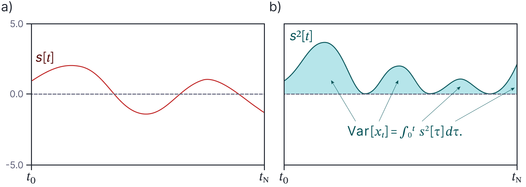
Figure 7. Variance of Wiener integral. a) Integrand $\mbox{s}[t]$. b) The variance of the integral is computed by squaring the integrand and computing a standard Riemann integral (i.e., computing the shaded area under the curve).
\begin{eqnarray}
\mathbb{E} \left[\int_0^t \textrm{s}\bigl[W_\tau,\tau\bigr] dw_\tau\right] &=& 0 \nonumber\\
\mbox{Var} \left[\int_0^t \textrm{s}\bigl[W_\tau,\tau\bigr] dw_\tau \right] &=& \mathbb{E} \left[\int_0^t \textrm{s}^2[W_\tau,\tau] d\tau\right].
\tag{13}
\end{eqnarray}
where the expectation is with respect to the Wiener process $W_{t}$.
Proof of Itô integral results
These results are important, so we’ll take a moment to prove them.
Proof of mean: We start from the definition of the Itô integral:
\begin{eqnarray}\label{eq:ode6_ito_integral_mean}
\mathbb{E}\left[\int_0^t \textrm{s}\bigl[W_\tau,\tau\bigr] dw_\tau\right] &=& \mathbb{E}\left[\lim_{N\rightarrow\infty} \sum_{n=0}^{N-1}\textrm{s}\bigl[W_{t_n},t_n\bigr]\bigl(W_{t_{n+1}}-W_{t_n}\bigr)\right]\nonumber \\
&=& \lim_{N\rightarrow\infty} \sum_{n=0}^{N-1}\mathbb{E}\Bigl[\textrm{s}\bigl[W_{t_n},t_n\bigr]\Bigr]\cdot \mathbb{E}\left[W_{t_{n+1}}-W_{t_n}\right]\nonumber \\
&=& \lim_{N\rightarrow\infty} \sum_{n=0}^{N-1}\mathbb{E}\Bigl[\textrm{s}\bigl[W_{t_n},t_n\bigr]\Bigr]\cdot \left(\mathbb{E}\bigl[W_{t_{n+1}}\bigr]-\mathbb{E}\bigl[W_{t_n}\bigr]\right)\nonumber \\
&=& \lim_{N\rightarrow\infty} \sum_{n=0}^{N-1} \mathbb{E}\Bigl[\textrm{s}\bigl[W_{t_n},t_n
\bigr]\Bigr]\cdot (0-0) \nonumber \\
&=& 0,
\tag{14}
\end{eqnarray}
where we have used the fact that the two terms are independent between lines one and two (so the expectation of the product becomes a product of individual expectation terms). Between lines two and three, we have used the property that the expectation of a sum is the sum of the expectations and between lines three and four, we have used the fact that the expectation of a Wiener process is zero.
Proof of variance: To prove the isometry property, we start once again with the definition of the Itô integral:
\begin{eqnarray}
\mathbb{E} \left[\left(\int_0^t \hspace{-2mm}\textrm{s}\bigl[W_\tau,\tau\bigr] dw_\tau\right)^2 \right]&=& \lim_{N\rightarrow\infty}\mathbb{E}\left[\left( \sum_{n=0}^{N-1}\textrm{s}\bigl[W_{t_n},t_n\bigr]\bigl(W_{t_{n+1}}\!-\!W_{t_n}\bigr)\right)^2\right]\nonumber \\
&=& \lim_{N\rightarrow\infty}\mathbb{E}\Biggl[ \sum_{n=0}^{N-1}\textrm{s}\bigl[W_{t_n},t_n\bigr]^2\bigl(W_{t_{n+1}}\!-\!W_{t_n}\bigr)^2\nonumber \\
&& +\!\!\!\!\sum_{i,j=0, i\neq j}^{N-1} \hspace{-0.3cm}\textrm{s}\bigl[W_{t_i},t\bigr]\textrm{s}\bigl[W_{t_j},t_n\bigr]\bigl(W_{t_{i+1}}\!-\!W_{t_i}\bigr)\bigl(W_{t_{j+1}}\!-\!W_{t_j}\bigr)\Biggr],
\tag{15}
\end{eqnarray}
where the first term in the final expectation contains the $N$ terms that are squares of the original constituents of the sum. The second term contains the remaining $N^2-N$ cross terms.
Once more we exploit the fact that an expectation of a product of independent terms is the product of expectations to yield:
\begin{eqnarray}
\mathbb{E} \left[\left(\int_0^t \textrm{s}\bigl[W_\tau,\tau\bigr] dw_\tau\right)^2 \right]&=&\\&&\hspace{-4cm}
\lim_{N\rightarrow\infty} \sum_{n=0}^{N-1}\mathbb{E}\Bigl[\textrm{s}\bigl[W_{t_n},t_n\bigr]^2\Bigr]\mathbb{E}\Bigl[\bigl(W_{t_{n+1}}-W_{t_n}\bigr)^2\Bigr]\nonumber \\
&& \hspace{-4cm}+\sum_{i,j=0, i\neq j}^{N-1} \mathbb{E}\Bigl[\textrm{s}\bigl[W_{t_i},t_n\bigr]\Bigr]\mathbb{E}\Bigl[\textrm{s}
\bigl[W_{t_j},t\bigr]\Bigr]\mathbb{E}\Bigl[W_{t_{i+1}}-W_{t_i}\Bigr]\mathbb{E}\Bigl[W_{t_{j+1}}-W_{t_j}\Bigr].
\tag{16}
\end{eqnarray}
Using a similar argument to that in the proof of the mean (equation 14), we see that $\mathbb{E}[W_{t_{j+1}}-W_{t_j}]=0$, and the second term becomes zero which leaves:
\begin{eqnarray}
\mathbb{E} \left[\left(\int_0^t \textrm{s}\bigl[W_\tau,\tau\bigr] dw_\tau\right)^2 \right]&=&
\lim_{N\rightarrow\infty} \sum_{n=0}^{N-1}\mathbb{E}\Bigl[\textrm{s}^2\bigl[W_{t_n},t_n\bigr]\Bigr]\mathbb{E}\Bigl[\bigl(W_{t_{n+1}}-W_{t_n}\bigr)^2\Bigr]\nonumber \\
&=& \lim_{N\rightarrow\infty} \sum_{n=0}^{N-1}\mathbb{E}\Bigl[\textrm{s}^2\bigl[W_{t_n},t_n\bigr]\Bigr]\mathbb{E}\biggl[ \Bigl(\textrm{Norm}[0, t_{n+1}-t_{n}]\Bigr)^2\biggr]\nonumber \\
&=& \lim_{N\rightarrow\infty} \sum_{n=0}^{N-1}\mathbb{E}\Bigl[\textrm{s}^2\bigl[W_{t_n},t_n\bigr]\Bigr](t_{n+1}\!-\!t_n)\mathbb{E}\biggl[ \Bigl(\textrm{Norm}[0, 1]\Bigr)^2\biggr]\nonumber \\
&=& \lim_{N\rightarrow\infty} \sum_{n=0}^{N-1}\mathbb{E}\Bigl[\textrm{s}^2\bigl[W_{t_n},t_n\bigr]\Bigr](t_{n+1}-t_n),
\tag{17}
\end{eqnarray}
where the expectation of the squared standard normal is the expectation of the $\chi$-squared distribution which is just one.
Looking at what remains, we see that we have a standard Riemann integral (as defined in equation 5):
\begin{eqnarray}
\mathbb{E} \left[\left(\int_0^t \textrm{s}\bigl[W_\tau,\tau\bigr] dw_\tau\right)^2 \right]&=& \int_0^t \mathbb{E} \Bigl[\textrm{s}^2\bigl[W_{\tau},\tau\bigr]\Bigr]d\tau\nonumber\\
&=& \mathbb{E}\left[\int_0^t \Bigl[\textrm{s}^2\bigl[W_{\tau},\tau\bigr] d\tau\right],
\tag{18}
\end{eqnarray}
where we have used Fubini’s theorem between the last two lines. The proof for the Wiener integral proceeds in exacly the same way, but without the need for the expectation term around $\textrm{s}^2\bigl[W_{\tau},\tau\bigr]$.
Surprising results
The previous section argued that the Itô integral is a random variable with mean zero and a variance that is computed using a Riemann integral. This immediately flags that the Itô integral must work differently from the Riemann integral. For example, consider the Riemann integral:
\begin{equation}
\int_0^{t} 2\tau \cdot d\tau = \tau^2 \biggr|_{0}^{t} = t^2
\tag{19}
\end{equation}
We can immediately see that the equivalent Itô integral:
\begin{equation}
\int_0^{t} 2 W_\tau \cdot dw_\tau.
\tag{20}
\end{equation}
will not evaluate to $W_{t}^2$ because $W_{t}^2$ is not a random variable whose expected value is zero. In fact, the result is given by $W_{t}^2-t$ (a shifted and scaled $\chi$-squared distribution). This can be proven by taking limits of the discrete integral in a similar way to that used in the proof of the mean and variance properties. The proof is provided at the end of this article for completeness.
Common examples of Itô integrals include:
\begin{eqnarray}
\int_0^t dw_\tau &=& W_t\nonumber \\
\int_0^t t\cdot dw_t &=& t W_t – \int_0^t W_{\tau} \cdot d\tau\nonumber \\
\int_0^t W_\tau\cdot dw_\tau &=& \frac{W_t^2}{2} – \frac{t}{2}\nonumber \\
\int_0^t W_\tau^2 \cdot dw_\tau &=& \frac{W_t^3}{3} – \int_0^t W_{\tau} \cdot d\tau.
\tag{21}
\end{eqnarray}
Additivity, homogeneity, and partition properties
In the last section, we saw that the rules governing stochastic integrals are not always the same as for Riemann integrals. However, the Itô integral does retain many of the properties associated with Riemann integrals. For example, it replicates the additivity, homogeneity, and partition properties.
Additivity: The Itô integral of a sum of terms is the sum of the individual integrals of those terms:
\begin{equation}
\int_0^t \bigl(\textrm{f}\bigl[W_\tau,\tau\bigr] + \textrm{g}\bigl[W_\tau,\tau\bigr]\bigr)dw_\tau =\int_0^t \textrm{f}\bigl[W_\tau,\tau\bigr]dw_\tau +\int_0^t \textrm{g}[W_\tau, \tau]dw_\tau.
\tag{22}
\end{equation}
Homogeneity: The Itô integral of a constant $a$ times a function $\mbox{f}[W_t,t]$ is the constant times the integral of $\mbox{f}[W_t,t]$ alone:
\begin{equation}\label{eq:ode6_homog}
\int_0^t a\cdot \textrm{f}\bigl[W_\tau,\tau\bigr] dw_\tau = a \cdot \int_0^t \textrm{f}\bigl[W_\tau,\tau\bigr] dw_\tau.
\tag{23}
\end{equation}
Partition property: The Itô integral from 0 to $t$ can be divided into the sum of the integral from 0 to $t'<t$ and the integral from $t’$ to $t$:
\begin{equation}
\int_0^t \textrm{f}\bigl[W_\tau,\tau\bigr] dw_\tau = \int_0^{t’} \textrm{f}[W_\tau,\tau] dw_\tau + \int_{t’}^t \textrm{f}\bigl[W_\tau,\tau\bigr] dw_\tau.
\tag{24}
\end{equation}
These properties follow naturally from the original definition of the Itô integral as the limit of a sum (equation 9).
Solving simple SDEs
Now that we understand the properties of the Itô integral, we can return to solving stochastic differential equations with the general form:
\begin{equation}\label{eq:ode6_general_sde2}
dx = \mbox{m}[x,t] dt + \mbox{s}[x,t] dw.
\tag{25}
\end{equation}
As for ordinary differential equations, these integrals are not always solvable in closed form, but there are special cases that can be handled.
Deterministic term zero, stochastic term one
In the previous article, we defined the solution for $\mbox{m}[x,t]=0$ and $\mbox{s}[x,t]=1$ to be the Wiener process. In other words, the solution to:
\begin{equation}
dx = dw
\tag{26}
\end{equation}
is:
\begin{equation}
x_t = x_0 + W_{t}.
\tag{27}
\end{equation}
Deterministic term zero, stochastic term constant
We can generalize this solution to the case where the drift term $\mbox{m}[x,t]$ is zero and the diffusion term $\mbox{s}[x,t]$ is a constant $\sigma$:
\begin{equation}
dx = \sigma \cdot dw.
\tag{28}
\end{equation}
Using the homogeneity property (equation 23), we can see that if $\int dw = W_{t}$, then $\int \sigma\cdot dw=\sigma\cdot W_{t}$ and so the solution is:
\begin{equation}
x_t = x_0 + \sigma \cdot W_{t}.
\tag{29}
\end{equation}
Deterministic term constant, stochastic term constant
By a similar logic to that above, we can solve an SDE where both the drift and diffusion terms are constant:
\begin{equation}
dx = \mu \cdot dt + \sigma \cdot dw.
\tag{30}
\end{equation}
The solution is given by:
\begin{equation}
x_t = x_0 + \mu \cdot t + \sigma \cdot W_{t}.
\tag{31}
\end{equation}
Terms are functions of time alone
Generalizing this equation somewhat further, we can consider the case where $\mbox{m}[x,t]=\mbox{m}[t]$ and $\mbox{s}[x,t]=\mbox{s}[t]$ are functions of time alone:
\begin{equation}
dx = \mbox{m}[t] dt + \mbox{s}[t] dt.
\tag{32}
\end{equation}
In this case, we can integrate the deterministic and stochastic parts separately and
\begin{equation}\label{eq:ode6_general_form2}
x_t = x_0+ \int_0^t \mbox{m}[\tau] d\tau + \int_0^t \mbox{s}[\tau] dw_\tau,
\tag{33}
\end{equation}
where the first integral is a Riemann integral and the second integral is an Itô integral. As long as these two integrals can be computed, this equation can be solved. The solution will be a stochastic process with a mean:
\begin{equation}
\mathbb{E}\bigl[x_{t}\bigr] = x_0 + \int_0^t \mbox{m}[\tau] d\tau,
\tag{34}
\end{equation}
and a variance given by the isometry property of the Itô integral:
\begin{equation}
\mbox{Var}\bigl[x_t\bigr] = \int_{0}^{t} s^2[\tau] d\tau.
\tag{35}
\end{equation}
Worked example
Consider the stochastic differential equation:
\begin{equation}
dx = \frac{1}{t+1}dt + \exp[at] dw.
\tag{36}
\end{equation}
Both terms depend on $t$ alone and so the solution to this integral comes from directly integrating:
\begin{equation}
I_t[x] = x_0+ \int_0^t \frac{1}{\tau+1}d\tau + \int_0^t \exp[a\tau] dw_\tau.
\tag{37}
\end{equation}
The result is a random variable with mean:
\begin{eqnarray}
\mathbb{E}\bigl[I_{t}\bigr] &=& x_0+ \int_0^t \frac{1}{\tau+1}d\tau \nonumber\\
&=& x_0 + \log[\tau+1]\biggr|_0^t\nonumber\\
&=& x_0 + \log[t+1],
\tag{38}
\end{eqnarray}
and variance:
\begin{eqnarray}
\textrm{Var}\bigl[I_{t}\bigr] &=& \int_0^t \bigl(\exp[a\tau]\bigr)^2 d\tau\nonumber\\
&=& \frac{1}{2a} \exp[2a\tau] \biggr|_0^t \nonumber \\
&=& \frac{1}{2a} \exp[2a t] – \frac{1}{2a}.
\tag{39}
\end{eqnarray}
Conclusion
In this article, we have investigated closed-form solutions for SDEs. We saw that when the drift and diffusion terms in the SDE depend only on the independent variable $t$, we can solve the SDE by directly integrating. However, the diffusion term is a stochastic (Itô) integral which has different properties from the standard Riemann integral. The result of the stochastic integral is a random variable, and we can derive expressions for its mean and variance.
In part VII of this series, we will see that when the drift and diffusion terms also depend on the dependent variable $x$, we can make progress by performing a change of variables, such that the new SDE has terms that only depend on $t$. We can then integrate as before and change the variable back again. To change the variable, we need Itô’s lemma, which we derive. We apply these ideas to solve the SDEs for geometric Brownian motion and the Ornstein-Uhlenbeck process.
Proof of Itô integral of Wiener process
This section proves the surprising result mentioned above:
\begin{equation}
\int_0^t W_\tau dw_\tau = \frac{W_t^2}{2} – \frac{t}{2}.
\tag{40}
\end{equation}
To prove this integral, we start by defining a discrete version:
\begin{eqnarray}
\int_{0}^{t} W_\tau dw_{\tau} &=&
\lim_{N\rightarrow\infty} \sum_{n=0}^{N-1}W_{t_n}\bigl(W_{t_{n+1}}-W_{t_n}\bigr)\\
&=& \lim_{N\rightarrow\infty} \sum_{n=0}^{N-1}W_{t_n}W_{t_{n+1}}-W_{t_n}^2\nonumber\\
&=& \lim_{N\rightarrow\infty} \sum_{n=0}^{N-1}W_{t_n}W_{t_{n+1}}-W_{t_n}^2 +\frac{1}{2}W_{t_n}^2-\frac{1}{2}W_{t_n}^2\nonumber\\
&=& \lim_{N\rightarrow\infty} \sum_{n=0}^{N-1} W_{t_n}W_{t_{n+1}}-W_{t_n}^2 +\frac{1}{2}W_{t_n}^2-\frac{1}{2}W_{t_n}^2\nonumber \\ && \hspace{6cm}+\frac{1}{2}W_{t_{n+1}}^2 -\frac{1}{2}W_{t_{n+1}}^2,
\tag{41}
\end{eqnarray}
where we have just added and subtracted identical terms in the last two lines. Extracting the factor $1/2,$ collecting terms and re-arranging, we have:
\begin{eqnarray}\label{eq:ito_noise_integral_terms}
\int_{0}^{t} W_\tau dw_{\tau}
&=& \lim_{N\rightarrow\infty} \sum_{n=0}^{N-1} \frac{1}{2}\left(W_{t_{n+1}}^2 -W_{t_n}^2\right) – \frac{1}{2}\left(W_{t_{n+1}}^2 -2 W_{t_n}W_{t_{n+1}}+W_{t_{n}}^2\right) \nonumber\\
&=& \lim_{N\rightarrow\infty} \sum_{n=0}^{N-1} \frac{1}{2}\left(W_{t_{n+1}}^2 -W_{t_n}^2\right) – \frac{1}{2}\bigl(W_{t_{n+1}} -W_{t_{n}}\bigr)^2.
\tag{42}
\end{eqnarray}
We’ll treat each of these terms in turn.
Term 1: Starting with the first term, we have:
\begin{eqnarray}
\lim_{N\rightarrow\infty} \sum_{n=0}^{N-1} \frac{1}{2}\left(W_{t_{n+1}}^2 -W_{t_n}^2\right) &=& \lim_{N\rightarrow\infty}\frac{1}{2}\left(W_{t_{N}}^2 -W_{t_0}^2\right) \nonumber \\
&=& \lim_{N\rightarrow\infty}\frac{1}{2}\left(W_{t}^2 -W_{0}^2\right) \nonumber\\
&=& \frac{W_{t}^2}{2},
\tag{43}
\end{eqnarray}
because by definition $W_{0}=0$, and the limit disappears as there are no remaining terms related to the interval $[t_n, t_{n+1})$ in the expression.
Term 2: Now we’ll address the second term from equation 42. It seems to be a random variable, so we can characterize it in terms of its first and second moments. The first moment is given by:
\begin{eqnarray}
\mathbb{E}\left[\lim_{N\rightarrow\infty}\sum_{n=0}^{N-1} -\frac{1}{2}\bigl(W_{t_{n+1}} -W_{t_{n}}\bigr)^2\right] &=&
\lim_{N\rightarrow\infty}-\frac{1}{2}\mathbb{E}\left[\sum_{n=0}^{N-1} \bigl(W_{t_{n+1}} -W_{t_{n}}\bigr)^2\right]\nonumber\\
&=&
\lim_{N\rightarrow\infty}-\frac{1}{2}\sum_{n=0}^{N-1} \mathbb{E}\left[\bigl(W_{t_{n+1}} -W_{t_{n}}\bigr)^2\right]\nonumber\\
&=&
\lim_{N\rightarrow\infty}-\frac{1}{2}\sum_{n=0}^{N-1} \mathbb{E}\left[W_{t_{n+1}-t_{n}}^2\right],
\tag{44}
\end{eqnarray}
where in the last line we have used the fact that $W_{t_2}-W_{t_1} = W_{t_2-t_{1}}$ because both $W_{t_2}-W_{t_1}\sim \mbox{Norm}[0,t_2-t_1]$ and $W_{t_2-t_1}\sim \mbox{Norm}[0,t_2-t_1]$. Substituting in this result, we have:
\begin{eqnarray}
\mathbb{E}\left[\lim_{N\rightarrow\infty}\sum_{n=0}^{N-1} -\frac{1}{2}\bigl(W_{t_{n+1}} -W_{t_{n}}\bigr)^2\right]
&=& \lim_{N\rightarrow\infty}-\frac{1}{2}\sum_{n=0}^{N-1} \mathbb{E}\Bigl[\mbox{Norm}[0,t_{n+1}-t_{n}]^2 \Bigr]\nonumber \\
&=& \lim_{N\rightarrow\infty}-\frac{1}{2}\sum_{n=0}^{N-1} (t_{n+1}-t_{n})\mathbb{E}\Bigl[\mbox{Norm}[0,1]^2 \Bigr]\nonumber \\
&=& \lim_{N\rightarrow\infty}-\frac{1}{2}\sum_{n=0}^{N-1} (t_{n+1}-t_{n})\nonumber \\
&=& -\frac{1}{2} (t_{N} – t_0) \nonumber \\
&=& – \frac{t}{2},
\tag{45}
\end{eqnarray}
where the final expectation term is the expectation of a $\chi$-squared distribution with one degree of freedom which is one.
Now let’s consider the variance. By a similar process, we have:
\begin{eqnarray}
\mbox{Var}\left[\lim_{N\rightarrow\infty}\sum_{n=0}^{N-1} -\frac{1}{2}\bigl(W_{t_{n+1}} \!-\!W_{t_{n}}\bigr)^2\right]
&=& \lim_{N\rightarrow\infty}-\frac{1}{2}\sum_{n=0}^{N-1} \mbox{Var}\Bigl[\mbox{Norm}[0,t_{n+1}-t_{n}]^2 \Bigr]\nonumber \\
&=& \lim_{N\rightarrow\infty}+\frac{1}{4}\sum_{n=0}^{N-1} (t_{n+1}-t_{n})^2\mbox{Var}\Bigl[\mbox{Norm}[0,1]^2 \Bigr]\nonumber \\
&=& \lim_{N\rightarrow\infty}\frac{1}{4}\sum_{n=0}^{N-1} (t_{n+1}-t_{n})^2\cdot 2 \nonumber \\
&=& \lim_{N\rightarrow\infty}\frac{1}{2}\sum_{n=0}^{N-1} (t_{n+1}-t_{n})^2\cdot
\tag{46}
\end{eqnarray}
where the final variance term is the variance of a $\chi$-squared distribution with one degree of freedom which is two.
Since we know that by definition $t_{n+1}-t_{n} = t/N$, we have:
\begin{eqnarray}
\mbox{Var}\left[\lim_{N\rightarrow\infty}\sum_{n=0}^{N-1} -\frac{1}{2}\bigl(W_{t_{n+1}} -W_{t_{n}}\bigr)^2\right]
&=& \lim_{N\rightarrow\infty}\frac{1}{2}\sum_{n=0}^{N-1} \left(\frac{t}{N}\right)^2\nonumber \\
&=& \lim_{N\rightarrow\infty} \frac{t^2}{2N}\nonumber \\
&=& 0.
\tag{47}
\end{eqnarray}
It follows that the second term from equation 42 is deterministic (i.e, the variance is zero) with value $-t/2$. Putting both terms together, we have:
\begin{equation}
\int_0^t W_\tau dw_\tau = \frac{W_t^2}{2} – \frac{t}{2},
\tag{48}
\end{equation}
as required.