
State of the art machine learning models can perform extremely well on experimental test data. However, they implicitly make the closed-world assumption; they assume that the data they will encounter in the real world is drawn from the same distribution as the train and test data. However, this is not always the case and for some inputs, it may not be sensible for the model to be applied at all.
For example, consider a natural language processing model that has been trained to classify restaurant reviews as having positive or negative sentiment. If the training data was in the English language, this model should not be applied if it receives input text written in Hungarian. To avoid this type of situation, it would be prudent to build a different system that can identify if a data example is suitable for the model to classify and reject it if this is not the case.
This type of problem is referred to as out-of-distribution or OOD detection; given a known dataset, the goal is to determine if a new sample belonged to the same distribution or is in some way atypical. An important assumption of OOD detection is that we do not have access to large numbers of the atypical samples. If we did, we could use supervised learning to classify each sample as belonging to the typical or atypical classes. Hence, OOD detection is usually applied when the OOD events are varied, rare, and their details remain unknown until they occur.
In part I of this two-part blog, we discuss the scenarios in which OOD data occurs and the applications of OOD detection. We then review a family of related OOD problems. The rest of this blog considers the case where we only have access to a clean set of input data and without associated labels and categorizes the various families of methods for this problem. In part II, we consider cases where we have (i) a clean set of data with classification labels, (ii) access to a small number of OOD examples, and (iii) a unlabelled mixture of clean and out-of-distribution data.
Background
In practice, OOD events usually occur in one of five scenarios:
- Unexpected inputs: The data may be unusual because of measurement errors, missing values, or data that has been erroneously included such as the English/Hungarian example above.
- Defects: The data sample is mostly typical, but there is a problem with a localized part. This is common in machine inspection applications.
- Malicious activity: There is a malicious actor who is deliberately trying to manipulate the output of the machine learning system by providing unusual inputs.
- Distribution shift: The distribution of the observed data changes over time, resulting in a decline in performance.
- Statistical outliers: If the original distribution is heavy tailed, then unusual samples will occasionally appear. While not technically OOD, it is difficult to ensure that a ML model can effectively handle all of these examples.
To some extent, the scenario may guide the OOD detection technique. For example, malicious inputs are by design very close to the true data examples, and defect detection requires us both to identify the sample as problematic and to localize the problem.
Applications
OOD detection has many applications but is often used when a bad decision could have drastic real-world consequences. For example, autonomous systems such as self-driving cars may frequently encounter new situations they have not been explicitly trained to deal with. Another example is medical imaging systems which are particularly vulnerable to OOD risks as they may receive inputs from a different modality, (e.g., MRI vs. CT scans), blurry images, or images taken from the incorrect direction. In these cases, the focus is on ensuring that the large system understands that it cannot make a sensible judgement for this data
A second situation is identifying malicious activity. This is usually infrequent, and the pattern changes over time as new methods of deception are tried. Examples of this are systems to detect network intrusion attacks and credit card fraud. Finally, there may be cases where we are actively seeking novelty for its own sake. For example, in video surveillance, the goal may explicitly be to identify unusual events. Similarly, in reinforcement learning, the agent may actively seek to explore areas of state space that is has not encountered before.
OOD Problems
The term “out-of-distribution detection” encompasses a family of closely-related tasks (figure 1 ).
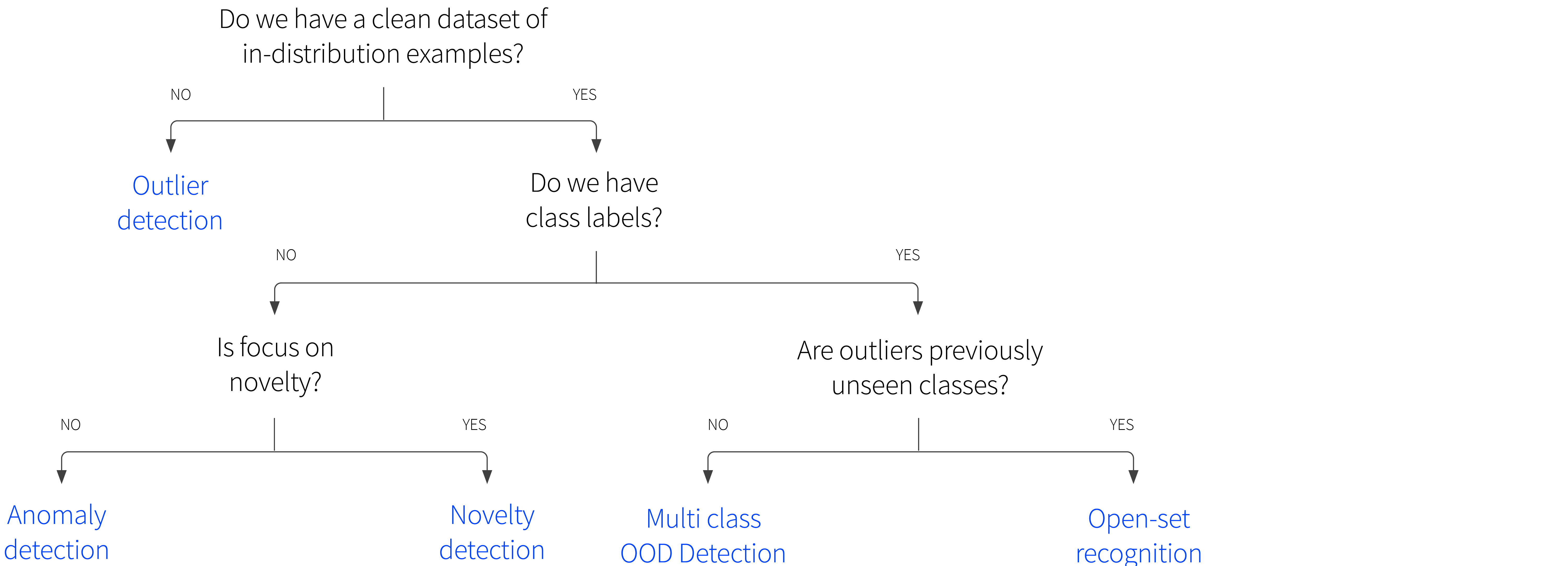
Figure 1. Flowchart showing relationship between OOD tasks.
Outlier detection: This problem is distinguished by the fact that we never receive a clean dataset containing only in-distribution examples. Instead, we receive an single unlabelled dataset $\{\mathbf{x}_{i}\}_{i=1}^{I}$ and wish to detect rare or low probability instances within it. Often these are due to noise, and the goal is just to identify and remove them before we use the data for some other purpose.
Anomaly detection: We receive an unlabelled dataset $\{\mathbf{x}_{i}\}_{i=1}^{I}$ consisting of only in-distribution examples. For a new example $\mathbf{x}^{*}$, we wish to identify if it belongs to the same distribution as the unlabelled dataset. In this situation, anomalies are often the quantities of interest, and represent examples that are erroneous, fraudulent, or suspicious. Examples might include industrial inspection, in which we aim to identify erroneous examples, or detecting suspicious credit card activity where we aim to identify fraudulent examples.
Novelty detection: We receive an unlabelled dataset $\{\mathbf{x}_{i}\}_{i=1}^{I}$ consisting of only in-distribution examples. For a new example $\mathbf{x}^{*}$, we wish to attach a score that indicates the novelty of the example. This is the same problem as anomaly detection, but without a final thresholding step. Moreover, the emphasis is different; here it is assumed that a novelty is an instance from some new region or mode of a non-stationary probability distribution, or at least something that we did not observe during training. Example applications might include finding novel news articles about a given company, or identifying novel states in reinforcement learning that should be explored.
Open-set recognition: We receive an labelled dataset $\{\mathbf{x}_{i},y_{i}\}_{i=1}^{I}$ where the labels $y$ come from a known predetermined set $\mathcal{C}$. We wish to determine which class $y^{*}\in\mathcal{C}$ a new example $x^{*}$ belongs to, or whether it belongs to another previously unseen class $y^*\in\mathcal{U}$. The usual scenario here is object classification and the unseen classes are semantic categories that we have not previously observed; for example, we may train a classifier to distinguish between species of birds. At test time we want to identify the species, but also flag if it seems to be a species that was not observed during training.
Multi-class OOD detection: We receive an labelled dataset $\{\mathbf{x}_{i},y_{i}\}_{i=1}^{I}$ where the labels $y$ come from a known predetermined set $\mathcal{C}$. We wish to determine which class $y^{*}\in\mathcal{C}$ a new example $x^{*}$ belongs to or whether it should not be classified. This is a very similar problem to open-set recognition, but the emphasis is different; here the non-typical data may be real examples that are corrupted or different in some way, rather than coming from an unseen class. For example, we may train a classifier to distinguish between species of birds. At test time we want to identify the species, but also flag images that are blurry, don’t contain birds, or the where view is very atypical (e.g., an extreme close up of the wing).
Note that these definitions are sometimes conflated or used inconsistently and so some caution is advised when consulting the literature.
OOD labels
A different way to partition the space of OOD problems is to consider the amount of labelled OOD training data available (figure 3 ). Arguably the most difficult scenario is outlier detection in which we do not have access to a clean in-distribution dataset, but only a dataset with outliers mixed in. Somewhat easier is the standard OOD scenario in which we have access to a clean dataset, but no outliers. This problem becomes slightly easier still if we have access to a few OOD examples, which we can exploit to calibrate or regularize our solution. Finally, with plentiful OOD examples the problem degenerates to a standard supervised learning task and doesn’t need specialized OOD methods.

Figure 2. Categorizing OOD problems by availability of OOD labels. Problems become easier from left to right. The hardest problem is outlier detection, in which we receive a mixture of in-distribution and out-of-distribution data with no labels. Following this, in decreasing difficulty, we may receive (i) a clean dataset of in-distribution samples (ii) a clean dataset plus a few labelled OOD examples, or (iii) plentiful labelled in-distribution and out-of-distribution samples.
OOD algorithms without class labels
In the remaining part of this blog, we will consider algorithms for anomaly/novelty detection. In other words, we’ll restrict our discussion to a situations where we have a clean dataset containing only in-distribution examples, but do not have access to either class labels or known OOD examples.
In this restricted scenario, there are seven main approaches to OOD detection:
- Classification: We use the clean dataset of in-distribution examples to build a one-class classifier that identifies if a new example belongs to the same dataset.
- Probability and generative models: We build a probability model of the in-distribution data and classify new examples with low probability as out-of-distribution.
- Typicality: We consider whether statistics of the input example are typical of the in-distribution data.
- Reconstruction: We learn an autoencoder that compresses in-distribution data to a low dimensional representation and then reconstructs it from this representation. Out-of-distribution examples are identified as those where the reconstruction quality is low.
- Auxiliary tasks: We build a model to perform an auxiliary task on the in-distribution data; for example, it might learn to rotate an in-distribution image to the correct orientation. For an OOD example, the performance on this task will be poor.Model consistency: We build more than one model of the in-distribution data; these models should react similarly to in-distribution data, but behave differently for out-of-distribution data.
We’ll now discuss each of these approaches in further detail.
Classification
Classification-based OOD methods define a boundary surface around the cloud of in-distribution data points. This surface should include all of the in-distribution examples while enclosing as small a volume as possible. New examples, are classified as OOD if they fall outside this volume. As with all classifiers, it is critical that the model has good inductive bias; we could define a trivial classifier of this kind by just thresholding the distance to the nearest data example, but this might not classify new points well in practice.
In early work, Schölkopf et al. (1999) used a single class support vector machine to find the tightest hypersphere around the data. New samples are considered outliers if they do not lie within this hypersphere (figure 3 ). However, with a simple kernelized formulation, this model cannot describe complex datasets such as images of cats. Consequently, Ruff et al. (2018) apply the same idea in a feature space created by a deep network. This network is carefully modified so that it cannot produce degenerate solutions where all the examples are projected to a point.
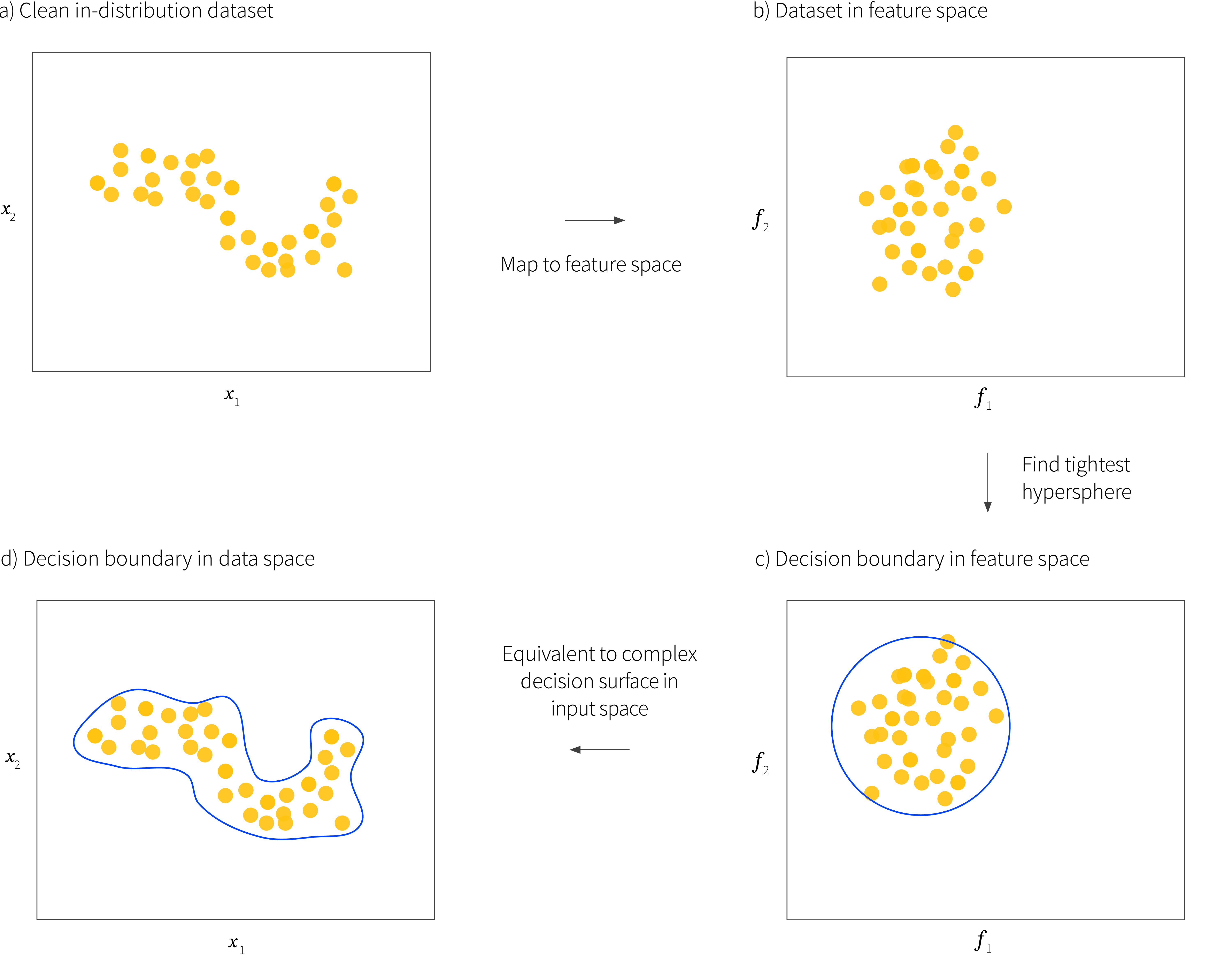
Figure 3. Classification approach. a) The system is provided with a clean set of in-distribution examples. b) These are mapped to a feature space using either kernel techniques or a deep network. c) The tightest possible hypersphere is fit to the data in feature space. This forms a decision surface and points outside it are considered out-of-distribution. d) This implicitly defines a complex decision surface in the original space.
Probability and generative models
Another simple approach is to build a probability model of the clean in-distribution data. New data points can be identified as OOD based on the measured likelihood under this model (figure 4). Early work in this area used parametric distributions, mixture distributions, and non-parametric approaches such as kernel density estimation. However, none of these methods can accurately describe the probability density of large high-dimensional datasets.
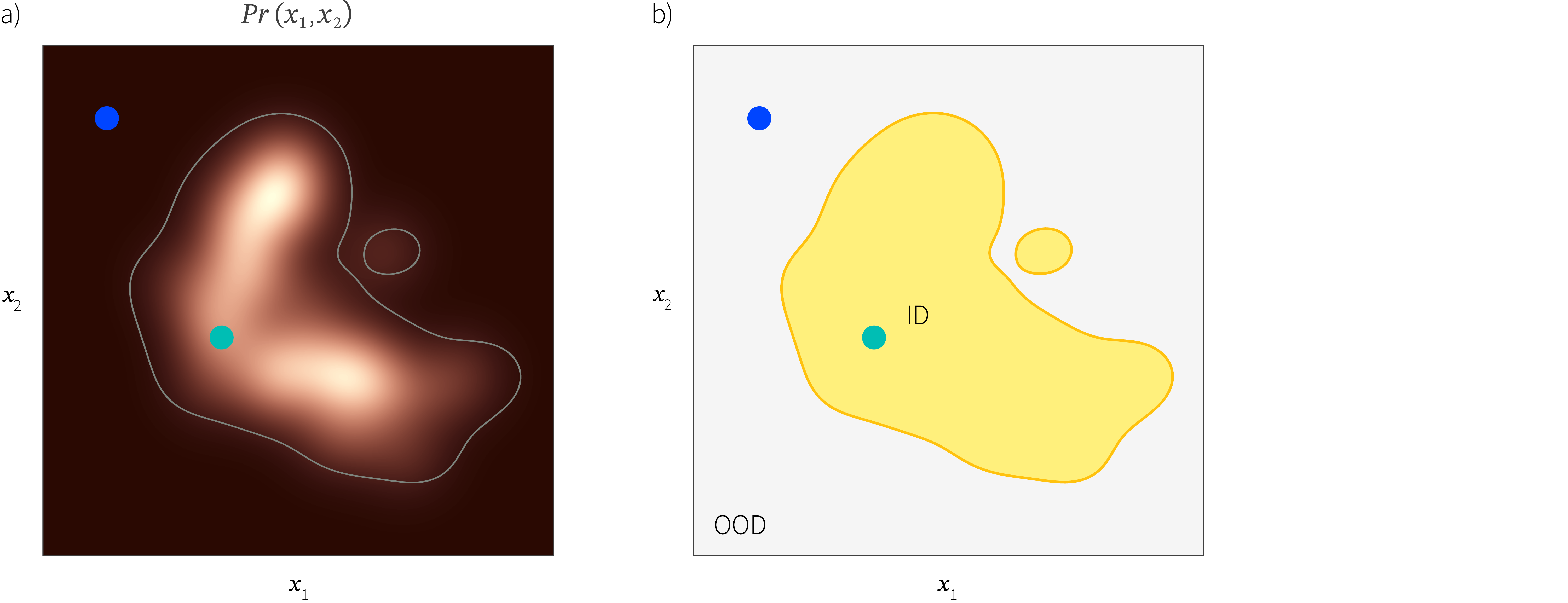
Figure 4. Probability approach. a) A probability model $Pr(\mathbf{x})$ is constructed from a training set $\{\mathbf{x}_{i}\}$ of clean in-distribution data. Heatmap represents probability density. If the probability is below a fixed threshold then we consider the example as out-of-distribution. b) This creates a decision boundary, so the blue point would be considered out-of-distribution and the green point would be considered in-distribution.
Fortunately, there now exist more sophisticated probability models based on deep-learning, and many of these have been applied to OOD detection. For example, Nalisnick at al. (2018) explore the use of variational autoencoders, auto-regressive models, and normalizing flows for OOD detection. Pidhorskyi et al. (2018) use an adversarial autoencoder model and assume that the probability distribution factors into a component that depends on the position on the manifold and a second component relating to the distance from the manifold. Zhai et al. (2016) use a deep structured energy based model to describe the probability.
It is also possible to apply non-probabilistic models like generative adversarial networks (GANs) along similar lines. Schlegl et al. (2017) exploit the idea that a generative model should have the capability of generating in-class examples. Their method (AnoGAN) used a trained GAN and seeks the hidden variable that best reconstructs the sample using an optimization strategy. It then uses a pixel-level loss. ADGAN (Deecke et al. 2018) follows a similar strategy. Zenati etl al. (2018) use a bi-directional GAN that has an encoder to find the latent vectors which makes this process more efficient.
There is evidence that some probabilistic methods work well for detecting OOD examples in tabular datasets, but Nalisnick at al. (2018) show that neither VAEs nor normalizing flow models work well for OOD detection in images. There are several possible reasons for this.
- Kirichenko et al. (2020) note that these models concentrate on modeling the probability of low level features such as the correlations of nearby pixels, and that these are shared across many image datasets. They demonstrate that normalizing flows work much better for high-level semantic features that were computed by passing the images through a pre-existing network that has been trained on a different dataset.
- The model may be devoting much of its representational power to modeling the background statistics. For example, in images, the object of interest is presented against a background, and equivalently in text there are many high-frequency stop-words which have little bearing on the semantic meaning (Ren et al. 2019).
- For some models, it is not possible possible to accurately evaluate the likelihood of a data point. For example, in VAEs we can make a point estimate of the hidden variable for the data sample and then evaluate the conditional likelihood, or compute the lower bound. However, neither of these is the correct probability estimate (Bütepage et al. 2019), which should be computed by integrating over the hidden variable. The data space with the highest likelihoods are vanishingly rare and are never observed during training. For example, consider a standard normal distribution in high dimensions; the highest probability is of course at the origin, but almost all real samples occur at a typical distance from the origin (figure 5). Nalisnick et al. (2018) identified that this phenomenon does indeed occur for VAEs, normalizing flows, and PixelCNN models. When trained on the CIFAR-10 dataset of image classes, these models all assign higher likelihoods to the (OOD) SVHN dataset of house numbers than to the test examples from the class they were trained on (figure 6).

Figure 5. Typicality. a) Consider sampling from a two-dimensional standard normal distribution (heatmap). For each sample (blue points) we compute the distance to the mean of the distribution (arrows). Consider bands spaced at equal distances from the center (i.e., between adjacent circles). Although the probability is highest close to the center, the area of these bands grows as we move further from the center. b) Consequently, when we plot the histogram of the distances of samples, very few are actually close to the center, and the typical distance from the mean is $\sqrt{2}$. c) This effect is exacerbated in higher dimensions. For example, for a standard normal distribution in 500 dimensions, it is very atypical for any sample will be a distance of less than 20 from the mean. Contrary to our expectations, the samples with the highest likelihood (near the mean of the distribution) virtually never occur in practice.

Figure 6. Likelihoods for a normalizing flows model trained on CIFAR10 image data. The test set of data has a similar distribution of likelihoods as the training set. However, the SVHN data (which consists of a completely different, but visually simpler class of image) has on average higher likelihood. It follows that likelihood is not a good criterion to identify OOD examples in this model. Adapted from et al. (2019).
Typicality and complexity
This notion of typicality is closely related to the complexity of the data; Serrâ et al. (2019) provide evidence that complexity dominates probability calculations and that simpler data examples tend to have higher probabilities even when OOD (figure 7). There are thus two obvious directions to take; either we base our decision on typicality directly, or find a way of factoring out the effect of complexity.
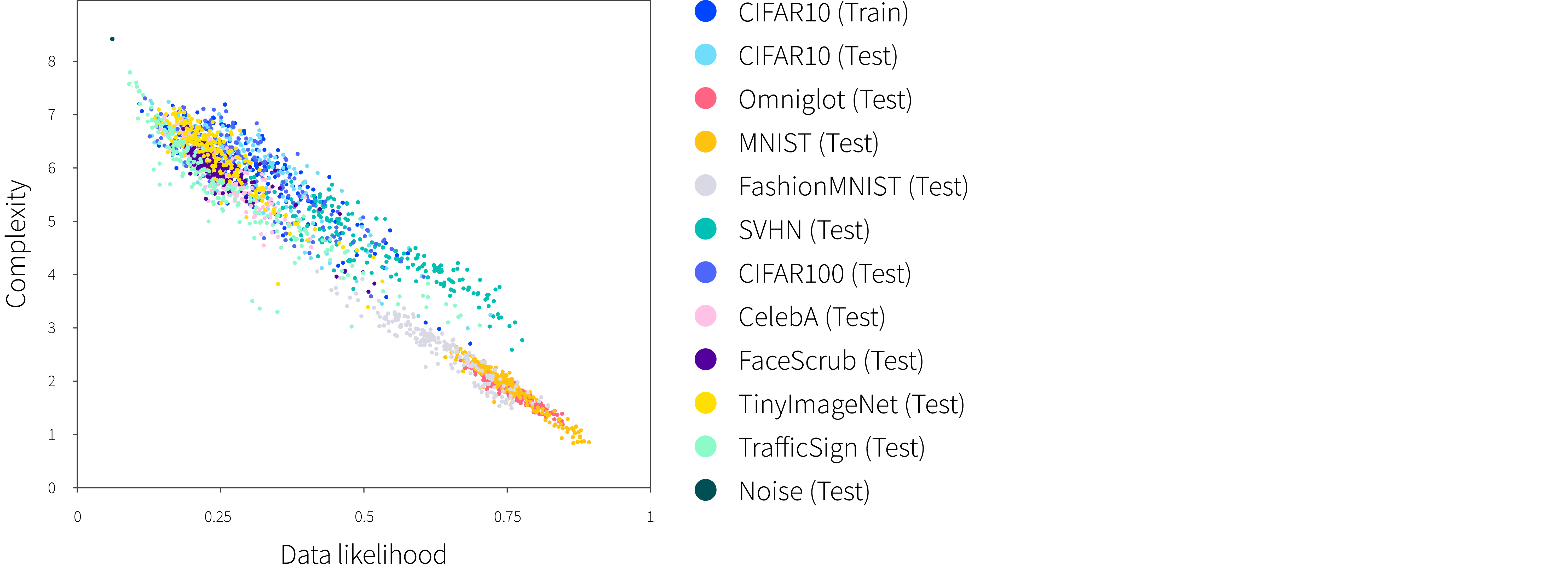
Figure 7. Relationship between likelihood and image complexity. The likelihood of data under an auto-regressive model of images is inversely correlated with the complexity of the image (as estimated by measuring the size of the compressed image). Similar results were observed for a normalizing flows model. Adapted from Serrâ et al. (2019)
Estimating typicality: Nalisnick et al. (2019) exploit typicality rather than probability to classify examples. They compare the average log likelihood of their dataset with the average log likelihood of a batch of new data and classify this batch as OOD if these differ by a wide margin. This method has the disadvantage that the performance degrades for single examples. Morningstar et al. (2020) take this idea one step further by computing multiple statistics (including log probability) for the true data and modeling the distribution of these statistics with independent kernel density estimators. This density of states model essentially uses the probability of the data probability (and other statistics) as a criterion for deciding whether an example is OOD.
Factoring out complexity: Serrâ et al. (2019) estimate the complexity of images using the size of the image after being passed through a PNG compressor. They show that that complexity is strongly anti-correlated with the probability under a PixelCNN model (figure 7). This leads to the simple idea of using the ratio between the probability and the complexity estimate as a criterion for OOD detection. This eliminates data complexity as a confounding factor.
An alternative approach to factoring out complexity is to explicitly build two probability models and use the ratio of the likelihoods as a criterion for OOD detection. To this end, Ren et al. (2019) suggest that in many cases data examples are divided into semantically meaningful (foreground) and semantically meaningless (background) parts. They then propose to build two models; the first describes the original images (containing foreground and background) and the second just the background distribution. They then use the likelihood ratio of these two models as a criterion for OOD detection. To create a dataset consisting of only background examples, they perturb the original data in such a way as to make it semantically meaningless. Simple OOD examples have high probability under both models and so the effect of complexity is cancelled out. Ran et al. (2020) adopt a similar approach in the context of variational autoencoders.
Reconstruction based methods
Another way to identify OOD examples is to build an autoencoder model for the dataset. This model learns to compress in-distribution examples to a low dimensional representation, and then to reconstruct them from this representation. It is posited that the autoencoder will (i) reconstruct the in-distribution examples well, but (ii) reconstruct out-of-distribution examples poorly. It follows that by thresholding the reconstruction quality, we can identify OOD data (figure 8).

Figure 8. Reconstruction based methods. An autoencoder is trained to reconstruct images of the digit eight. The theory is that it will be able to reconstruct new images of the digit eight well, but will reconstruct OOD examples poorly. In practice, the basic autoencoder structure does not ensure that OOD examples won’t be reconstructed well and so various extensions have been proposed. The reconstruction error may be combined with a probability model in the latent space, or an estimate of sparsity. The latent space may be manipulated so it can only reconstruct the training class, or the reconstruction error criterion can be replaced with a classifier. Results from Perera et al. (2019).
Note that for the variational autoencoder, this is very similar to basing our decision on the likelihoods, and indeed this approach suffers from the same problems as probabilistic methods. While it’s certainly true that the model can reconstruct in-distribution examples well, it does not necessarily imply that it will reconstruct out-of-distribution examples badly. This is especially the case when the out-of-distribution examples are simpler than the in-distribution examples.
However, the use of the autoencoder structure permits us to exploit the statistics of the latent representation as well as the statistics of the raw data. To this end, Abati et al. (2019) built a system that requires both good reconstruction, and that the latent representation has high probability over under a learned auto-regressive model. Similarly, Zong et al. (2018) learn a Gaussian mixture model that describes a joint distribution over both the reconstruction error and the hidden space. This gives a single criterion that will return a low value if either the reconstruction error or the position in encoding space is unusual. These methods can be thought of as combining reconstruction and probabilistic approaches.
A similar approach is train the autoencoder to produce sparse representations in latent space for in-distribution data, and use sparsity as an additional test to determine if the sample is OOD; the model may not be able to reconstruct OOD data from a sparse representation. All of these approaches can also be considered as combining reconstruction with a notion of typicality; the latent representation likelihood or sparsity can be thought of as a statistic of the data example that is evaluated for how typical it is.
A different line of work considers constraining the properties of the latent space to ensure that it can only reconstruct in-distribution examples. Gong et al. (2019) force the input to the decoder to be a sparse combination of learned prototypes. In this way, they effectively project an arbitrary point in the hidden space onto a manifold that is known to reconstruct the class well. Perera et al. (2019) attack the same problem in a different way by imposing terms in the cost function that ensure that (i) the distribution in the latent space is uniform and (ii) that random samples drawn from it are indistinguishable from real samples.
A third family of approaches uses autoencoders, but uses the classifier from generative adversarial network (GAN) to make the OOD decision. For example, Sabokrou et al., 2018 train a denoising autoencoder network to reconstruct in-distribution examples that have had noise added to them. This is trained with a GAN loss where the GAN tries to distinguish a reconstructed example from a true one. During testing, either the discriminator alone is used to detect if this is true example, or the image is passed through the autoencoder first which reconstructs well for true examples, but badly for outliers. Somepalli et al. (2021) and Zaheer at al. (2000) present variations on this idea.
Auxiliary tasks
A completely different approach to OOD detection is to train a network to perform an auxiliary task on the in-distribution data. Since we do not have any associated labels, this task must be self-supervised. For example, we might ask the network to fill in parts of the data that have been withheld, or to transform the image back into a canonical position. The trained network should be able to accomplish this task for in-distribution data, but will be unable to for out-of-distribution data.
Liu et al. 2018 build an image-to-image model based on the U-Net architecture which aims to predict the next frame in a sequence of surveillance images using an adversarial loss to ensure that the predictions are visually realistic. Their decision criterion is based on the idea that if a novel event occurs, the difference between the predicted and real frame will be large (figure 9). Along similar lines, Ravanbakhsh et al, 2019 use an image-to-image task in which they attempt to predict the motion of a frame of surveillance video from the raw-pixel data and vice-versa in a GAN setting. They use the discriminator from the GAN to determine if the output is a real pair or was generated.
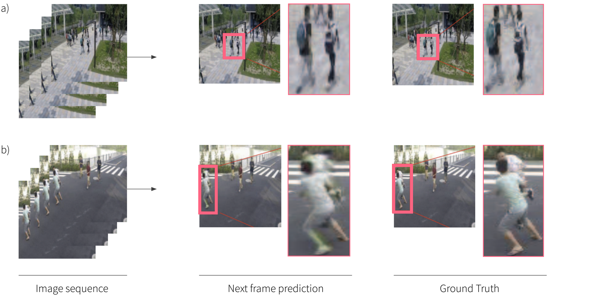
Figure 9. Ancillary tasks. A network is trained to perform a task on in-distribution data. For example, Liu et al. 2018 built a system to predict the next frame in a sequence. a) When the input sequence is typical, the predicted frame is close to the ground truth. b) When the input sequence is anomalous (here two men fighting) there are notable reconstruction errors including blurring and color changes. Adapted from Liu et al. 2018.
Golan and El-Yaniv (2018) trained a classifier to identify which of 72 transformations had been applied to the original image. This classifier returns a categorical distribution over the 72 entries and this is compared to a Dirichlet distribution over these 72 entry histograms generated from in-distribution data. For out-of-distribution data, the system cannot reliably estimate which transform has been applied. For example, if it has never seen a picture of a face before, it cannot know its canonical orientation.
Tack et al. (2020) use the same principle in a completely different way. The build upon SimCLR which is an unsupervised learning approach that attempts to make the data representation invariant to transformations, while maintaining differences between individual samples. Their criterion is built upon the principle that in this space transformed examples of in-distribution data will lie close to one another, bot transformed examples of out-of-distribution data will not.
Consistency
A final strand of work considers consistency between models; if we train multiple models using in-distribution data, we expect them all to behave similarly for a test set of in-distribution data, but they may behave very differently for out-of-distribution data. Essentially, this exploits the idea that extrapolation from any dataset is unreliable. For example Choi et al. (2018) build multiple generative models of in-distribution data and base their OOD decision on the Watanabe-Akaike information criterion. This favors cases where the log likelihoods of the models are high on average but have low variance.
Conclusion
In this blog, we motivated out-of-distribution detection and presented a taxonomy of related tasks. We then considered six families of methods for the simplest case, in which we have access only to a clean dataset of in-distribution samples. These methods were based on classification, modeling likelihoods, considering typicality, reconstruction, ability to solve auxiliary tasks, and consistency across multiple models. For further reading on OOD detection, consult the review by Yang et al. (2021). In part II of this blog, we will consider more complex scenarios where the dataset is not clean, or we have access to additional training data such as labels, or actual OOD examples.