
If you want to disrupt financial services with AI, you need to be the world’s expert on how to defend against AI risk. In this blog, we are going to be focus on one risk in particular, namely, Algorithmic Discrimination. There are three main research challenges associated with this problem: first is to identify sources of the bias and understand how models are influenced by them. The second is to redesign training algorithms to prevent unfair behaviours from being learned. The final challenge, which we address today, is to test the fairness of existing ML models.
We’ll begin by looking at some mechanisms by which models learn to discriminate, how we can design tests to catch this behavior, and finally how measure the reliability of fairness tests.
Mechanisms of Discrimination
Let’s start with a seemingly simple question: when is a model “good?” From the training perspective, a “good” model is one that maximizes/minimizes a certain performance metric (such as accuracy). But for a model with potentially billions of parameters, how can you possibly summarize behaviour with a single number? There are MANY settings of the parameters that will result in the same high accuracy score. How do we know that those parameters translate to desirable behaviour? How do we know that that the model’s decisions are justified?
Consider a simple example. What do you see in the image below? Perhaps you spot a triangle that reminds you of a sail, and a long thing rectangle that reminds you of a mast, and you conclude that this is a picture of a boat. Indeed, if I feed this into a convolutional neural network, it will also predict a boat. However, if you examine what the model is paying attention to, you’ll find it completely ignored all of the features you spotted. It just pays attention to the colour of the background! The dataset has a bias – namely, that all pictures of boats have blue backgrounds – and it has used this bias to “cheat” on its inference obtain a high accuracy.

Figure 1: Illustration: CNNs can exploit colour biases to inform their predictions. Taken from [1].
Now you can imagine, based on the introduction, that this isn’t a phenomenon that’s unique to boats. Indeed, our datasets contain many different social biases as well, and these must be considered before using algorithms in the real world. Below is another example of an image dataset in which the target is occupation. The dataset has a gender bias, and much like the boat example, a model trained without regularization will leverage this to inform its predictions. You can see this from the attention maps pictured pictured below: images of female doctors are is classified as nurses! The model justifies this prediction with gendered information, such as facial features, that are highlighted in red. In contrast, for a regularized model, the resulting attention maps are concentrated on equipment, rather than facial features.

Figure 2: CNNs can take advantage of other biases too. Taken from [2].
What’s going on here? Why pick one set of features over another? In the examples we’ve looked at, we’ve seen that the a single dataset can, in a certain sense, contain multiple “patterns” inside of it. Let’s be more formal, and define some variables:

Figure 3: Graphical models depicting patterns of bias.
- First, we have our training inputs, $X$, which consists of all those images of doctors and nurses.
- Inside the image there is some relevant source of variation we want to capture, say, occupation. These form our targets, $Y$.
- There are a number of irrelevant degrees of freedom, such as pose and lighting. These are unlabelled latent factors, $Z$.
- Finally, there are also sensitive, protected demographic variables, such as race and gender. Let’s call this $C$.
If the dataset were unbiased, there’d be only a single path from $X \rightarrow Y$ . However, the presence of bias produces an association between $Y$ and $C$, which creates a second pathway $X \rightarrow C \rightarrow Y$ . Now you can see the danger of training with a single performance objective: if we only optimize for accuracy, the model is free to choose the inference path! Before we can release algorithms into the real world, we need to find a way to catch models that are exploiting biases. We do this through fairness testing.
Fairness Definitions
Defining fairness is not easy – there’s more than twenty different ways, and many of them are mathematically incompatible [3]. In this section, we’ll take a look at two ways to analyze fairness: at the global level, and at the individual level.
Group Fairness
One way to examine fairness is at the global level. The idea is to statistically quantify disparate treatment by aggregating results across a whole population. Fairness testing is then based on testing criteria for the distribution of positive/negative outcomes. These are easy to implement, and you can compute them without access to the original model – because you only needs its predictions, you can even test historical data.
One example of a fairness criteria is independence: the score of a model should be statistically independent of a population. We can test this by computing demographic parity, which stipulates that the the same proportion of each population should be classified as positive. We illustrate an example below. On the right are the distribution of scores for a credit model, and by picking a threshold (the black vertical line), we can the score into a binary decision $\hat{y}$. As you can see from the bar graph on the right, the blue population is disadvantaged, so that demographic parity is violated.
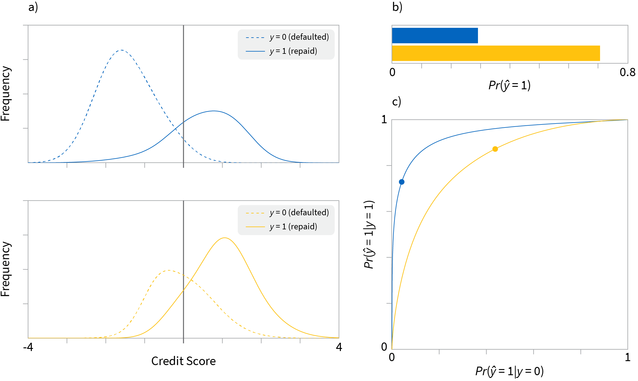
Figure 4: Testing a credit model using demographic parity.
While intuitive, there are a number of difficulties with group fairness tests:
1. They offer no insight into underlying mechanisms of discrimination.
2. They are limited to previously-seen datapoints – which means, while we can test if the model is fair on data we’ve seen, we can’t really tell if it will be fair in the future.
3. Finally, we cannot determine whether or not specific individuals – or indeed, a certain subpopulation – have been treated unfairly.
If any of the above concerns are important to you, you need to keep reading.
Individual Fairness
The above limitations of group fairness can be addressed by considering individual fairness. Here again, there are multiple definitions, but there is an underlying theme: similar individuals should be treated similarly.
A particularly simple idea is that models should be “blind” to the protected variable: either it is insensitive to perturbations, or it’s simply not included as part of the dataset. However, this definition ignores several mechanisms of discrimination! Indeed, as we’ve already shown, models can still learn to discriminate by leveraging correlations. Those correlated variables can be used as surrogates for the protected variable!
Another approach, Fairness Through Awareness (FTA) [4] formalizes the notion of “similar” using task specific metrics. In effect, fairness is a (D, d) Lipschitz property which bounds how different a model’s outputs can be for two individuals who are nearby each other:
\begin{equation}
D(f(x_1), f(x_2)) \leq d(x_1, x_2) \tag{1}
\end{equation}
Discrimination is flagged when, for a given individual x, you can find another individual x ′ that gets treated substantially differently. This is somewhat similar to an adversarial attack on the model. Formally, discrimination occurs when:
\begin{equation}
\exists \textbf{x}^{\prime} \,s.t \, \left(d(\textbf{x}, \textbf{x}^{\prime}) \leq \epsilon \right) \land
\left(D(f(\textbf{x}), f(\textbf{x}^{\prime})) > \epsilon \right) \tag{2}
\end{equation}
This definition has its own problems: beyond needing pairwise comparisons (which don’t scale), these task specific metrics often require experts to specify. With the wrong choice of metric, the test could be sensitive to more innocent variations in the data.
How do we identify what are the correct, sensitive variations? One answer is provided by Counterfactual Fairness (CFF). Loosely, the idea is to consider searching for disparate treatment inside of a fair “subspace.” Consider the figure below:
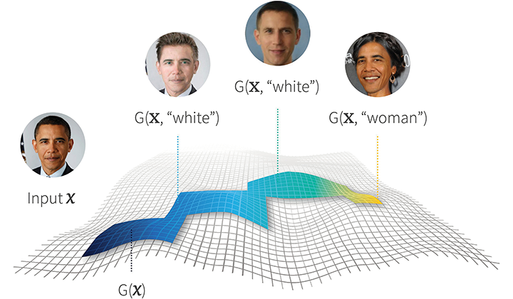
Figure 5: Counterfactual fairness.
In this figure the input X is generated by a collection of latent variables. If we modify only the protected variables (such as race and gender), we will generate new inputs, called counterfactuals. These individuals are all “similar” in that all the latent variables remain unchanged. Accordingly, the predictions of a fair model should also remain unchanged.
The tradeoff is that, if a causal graph is not available (they rarely are), you have to construct one. This involves substantial model overhead. It is is essentially generative modelling, which is not an easy task. Depending on the algorithm you use, and especially when the inputs are high-dimensional, a lot of the modelling effort will go into reproducing irrelevant factors of variation (those Z’s from before). What’s more, this more complicated model can fail in all sorts of new ways: you might generate many out of distribution samples, or produce only a small number of viable samples!
What we need is a method that is sensitive to surrogate features, insensitive to irrelevant perturbations, and involves low modelling overhead. What can be done?
fAux: Auxiliary models
Let’s consider making very small changes inside of that protected subspace. In Calculus, the change in a function when we only perturb one variable is given by the partial derivative. Thus, we can bound the change in the model’s decisions by bounding the partial derivative:
\begin{equation}
\begin{aligned}
%\max_{k}
\left|\frac{\partial f_{tar}( \mathbf{x})}{\partial \mathbf{c}}\right|_{\infty}
\leq \delta,
\end{aligned}
\label{eq:local_independent_definition} \tag{3}
\end{equation}
Now, the target model f is not an explicit function of the protected variable c, so we need to use the chain rule:
\begin{equation}
%\max_k
\left|\frac{\partial f_{tar}( \mathbf{x})}{\partial \mathbf{x}} \frac{\partial \mathbf{x}}{\partial \mathbf{c}}\right|_{\infty} \leq \delta. %\lim{\Delta{\mathbf{c}}\to 0}\frac{\delta}{\Delta{\mathbf{c}}},
\label{eq:chain_rule_expansion_lic} \tag{4}
\end{equation}
Our final result involves a dot product between the gradient of our target model, and the local difference between an individual and their counterfactuals. Now, before we can use this formula, we that $\frac{\partial \mathbf{x}}{\partial \mathbf{c}}$ term. It turns out, however, that we do not need a generative model to estimate this! Instead, we can train an auxiliary model $f_{aux}$ to estimate the probability of belonging to a certain protected group. In contrast to CFF, this is just supervised learning!
To see how this works, consider that, when I make an intervention on $C$, the score output by the auxiliary model changes. Thus, we can use the score of this model as a surrogate for protected group membership. In effect, we want to keep as much about $x$ unchanged as possible, while maximizing the probability that x belongs to the other group. Intuitively, this allows us to estimate the partial derivative, because we are isolating the component of $x$ that varies only with the protected attribute. With a little calculus you can show this point is given as follows:
\begin{equation}
f_{aux}^{-1}(\mathbf{c}) =\mathbf{x}_0 + (\mathbf{c} – f_{aux}(\mathbf{x}_0))\left(\nabla f_{aux}^\top\nabla f_{aux}\right)^{-1}\nabla f_{aux}^\top %\nonumber
\label{eq:penrose-invers} \tag{5}
\end{equation}
One partial derivative later, and you have the following fairness test:
Algorithm 1: Auxiliary Model Test (fAux)
Result: Flag unfair model behaviour
Input: Validation data points $D = \{\cdots(\mathbf{x}_i, \mathbf{c}_i, y_i)\cdots\}$, target model $f_{tar}$, and threshold $\delta’$
Train auxiliary model $\mathbf{c}=f_{aux}(\mathbf{x})$;
for each data point $(\mathbf{x}, \mathbf{c}, y)$ in $D$ do
Evaluate gradients $\nabla f_{tar}$ and $\nabla f_{aux}$;
Flag unfair behaviour on inputs through $\left|\nabla f_{tar} \left(\nabla f_{aux}^\top\nabla f_{aux}\right)^{-1}\nabla f_{aux}^\top \right|_{\infty} \leq \delta’$;
end
We take a target model and a dataset, and use supervised learning to fit an auxiliary model. Then, using the gradients of both the target and auxiliary model, we compute an alignment score. If the score is greater than a user-specified threshold, we flag the target model’s decision as unfair.
Generating Realistic Synthetic Bias
Now that we have an algorithm, we need to make sure it works. But how can you measure the reliability of a discrimination test? We can analyze this by constructing synthetic datasets, for which we can control the amount of discrimination. If the test gives a high score when discrimination is high, and a low score when discrimination is low, the test is reliable! In this section, we’ll outline how to construct these synthetic datasets. We’ll begin with a simple demonstration, and then show how we can generalize to more complex examples.
Demonstration: Coloured MNIST
Consider the humble MNIST dataset, which consists black and white images of handwritten digits. We are going to inject a simple colour bias: let all 9’s be coloured red, and all 0’s be coloured blue. If we train a model to distinguish between 0’s and 9’s, it can cheat by just learning to distinguish between colours, instead of shapes. This much is revealed when we look at the gradients (depicted in the blue channel):
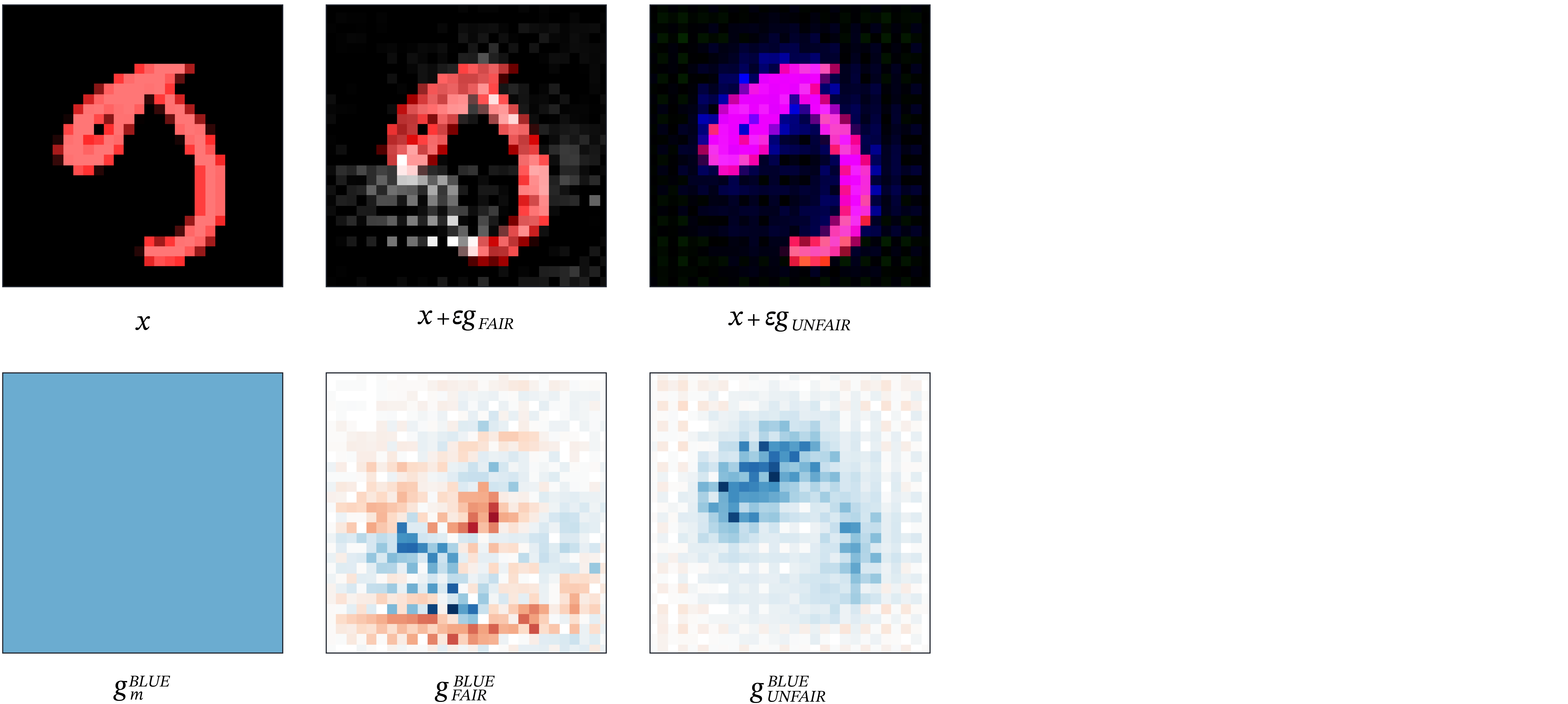
Figure 6: Comparing gradients Top row: counterexamples obtained by following model gradients.
Bottom row: comparison of the different gradients in the blue channel. Observe that the fair gradient
changes the shape of the digit, whereas the unfair gradient only changes its colour. The latter aligns
more closely with the gradient of the auxiliary model, which is evidence of its unfairness.
On the bottom left, you can see gradient of the auxiliary model, followed by the gradients of an unfair (unregularized) and a fair model. Instead of just computing the dot product, we can visually see the alignment by looking at what happens when you perturb the inputs using the respective gradients. Intuitively, these are the inputs that would maximize the probability of being classified as a 0 instead of a 9. We see that the fair model tries to “complete the loop” that turns the 9 into a 0. It’s learned information about shape. In contrast, the unfair model just changes the colour.
Now, the colour is a very simple pattern that can be learned by a linear model. We want to construct patterns of bias that are more noisy and nonlinear, indeed, so that they can be more similar to real datasets.
We can generalize this approach by using real datasets as the pattern of bias! We depict our pipeline beflow:
A general algorithm for synthetic datasets
In effect, you have two different datasets, for which we can construct generative models. One of these datasets is in a certain sense a “harder” learning task than the other. In our previous example, the digits were the hard problem, and the colour was the easy problem. The inputs of these datasets can be combined together via some function to produce the inputs for a “fused” dataset, which in the previous case, were the coloured digits. Call this second label C, and add some correlation between the labels of both datasets, and you can see that the resulting graph has the same structure as the biased graph we discussed in the introduction.
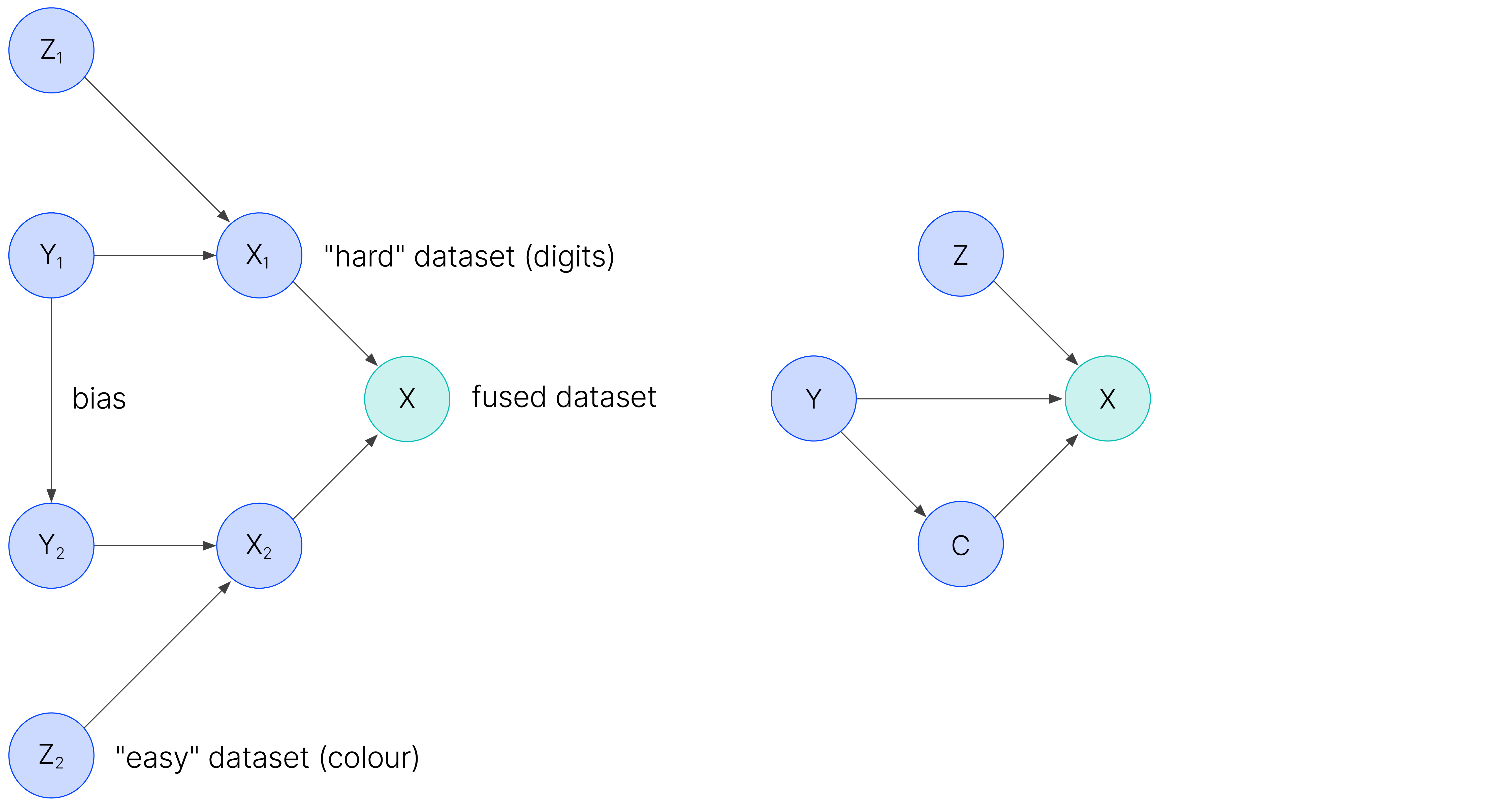
Figure 7: Synthetic data generation pipeline.
We expect any model trained on this dataset will learn to exploit the bias. Indeed, this is what we observe! You can see that in the histograms below. Because we have access to the generative models, we can evaluate a ground truth unfairness score using counterfactual fairness. The framework gives us a tuneable bias knob, and without regularization, more bias leads to more discrimination, no matter the architecture.

Figure 8: Our framework gives us tuneable knobs to control the amount of bias. Without regularization,
more bias leads to more discrimination, no matter the architecture.
Measuring accuracy of fairness tests
Having access to the generative model is really useful, because we can build models that are fair by construction. We also have access to the ground truth fairness score, which we can use to compare the accuracy of different fairness tests.
In the figure below, on the vertical axis we have that ground truth unfairness score, and on the bottom we have the predicted unfairness score from two tests. Decisions made by unregularized (unfair) models are denoted with white circles, and decisions made by fair models are denoted by black crosses. We see that both tests are able to recognize that the unfair decisions are unfair – however, FTA also gives a high unfairness scores to fair decisions! It turns out that this test is just very sensitive to models that have large gradients, as opposed to models that discriminate. In contrast, our test, fAux, is only sensitive to variations in the protected attribute: the fair predictions all receive a discrimination score of 0.

Figure 9: Comparing predicted and ground truth measures of discrimination for two different fairness
tests. On the left, fAux. On the right, Fairness Through Awareness using a euclidean distance metric.
How can we be more quantitative with our comparison? We’d like to identify how “accurate” the fairness tests are. To quantify how reliable a given fairness test is, we begin by thresholding the ground truth score, to obtain a binary label for discrimination. One approach would then be to threshold the predicted unfairness score, and compute the binary accuracy. In practice, this threshold is usually set by regulatory standards that depend on problem domain or statistics of manual auditing results. The selection of such a threshold is a subtle question, and in practice, decision-making may involve multiple thresholds that require further domain-specific study. Instead, we determine how reliable each test is across a range of different thresholds by looking at the precision-recall (PR) curve. More reliable tests will have larger areas under the PR curve.
In the table below, we compare the average precision scores of fAux against some other individual fairness tests in the literature. We see that fAux dominates the competition. For full details about these other tests, and the settings used in the experiments, we refer the interested reader to our paper.
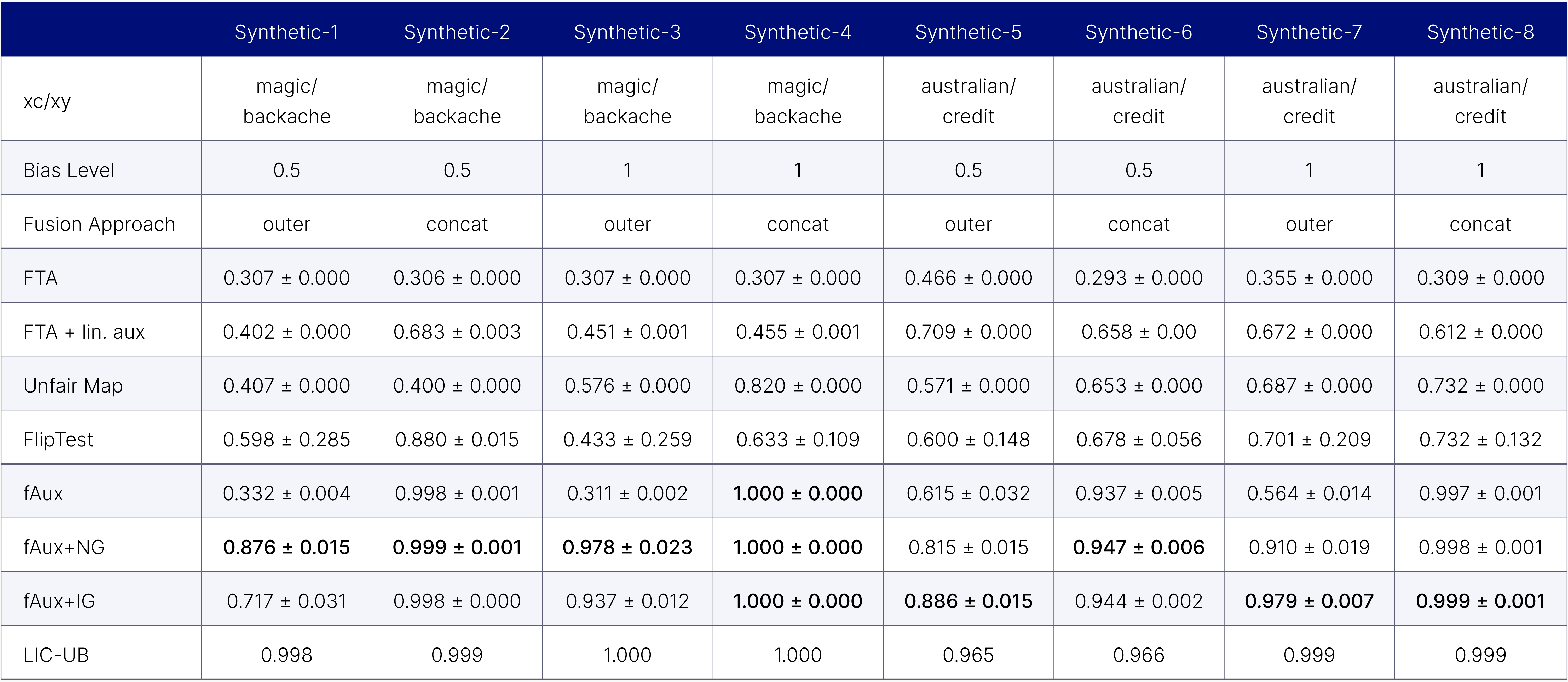
Table 1: Performance Comparison among Individual Fairness Testing Methods on Synthetic Datasets We report Average-Precision scores with the highest score in bold font. The confidence interval comes from 10 runs by re-training auxiliary models. Rows are sorted in order of increasing computational requirements. The last row corresponds to a theoretical upper bound.
Real Datasets
For real datasets, we don’t have ground truth labels for discrimination, thus we cannot quantify the precision of a fairness test at the level of individual datapoints. We will have to analyze the performance of fAux in other ways. In particular, we will look at:
- How does our test compare with other definitions of fairness?
- Can we distinguish between fair and unfair models?
- Given an unfair model, can we provide insight onto the mechanism of discrimination?
Let’s consider a standard dataset, the Adult Income dataset, compiled from census data. This dataset is often studied in the fairness literature as an example of a dataset biased against gender. Below you can see one analysis of the dataset which demonstrates how the features are related to one another:
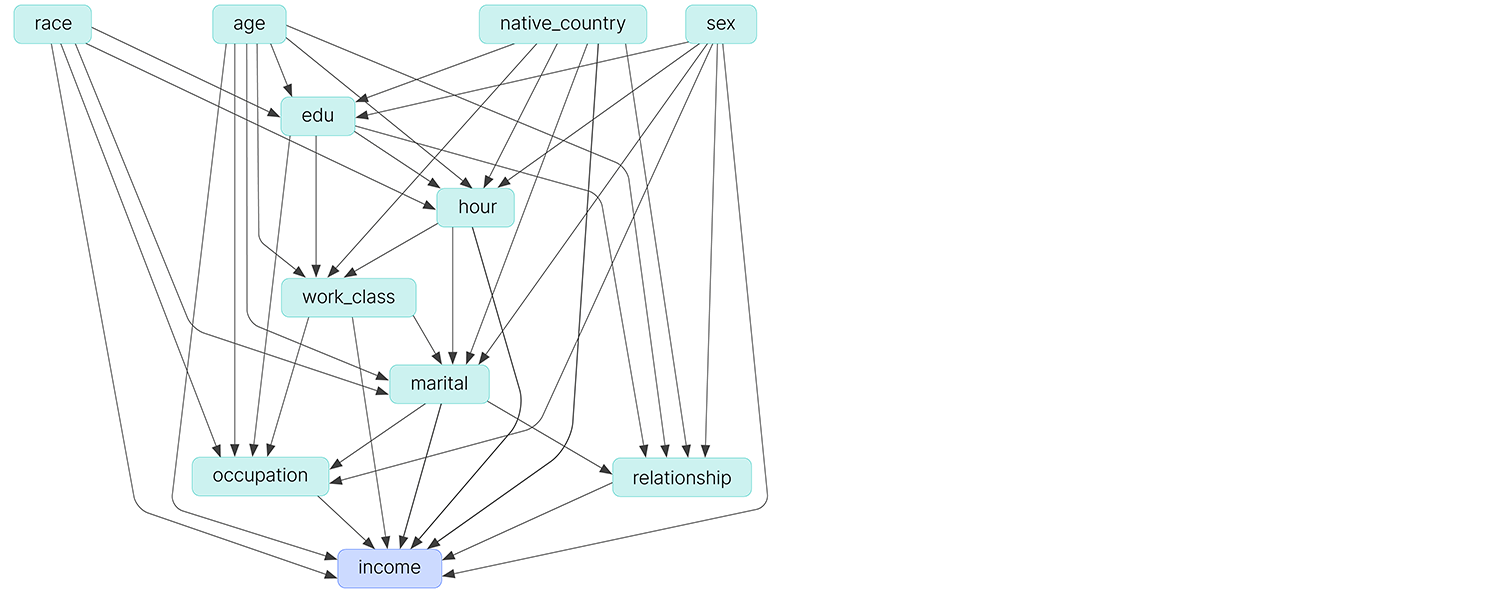
Figure 10: A candidate causal graph for the adult income dataset. Taken from [5].
We can see that the target here – income – is related to protected variables such as gender through features such as “occupation” and “marital status.” This is problematic, because datasets of this sort are often used to train credit score models. Accordingly, we will want to make sure a potential credit model does not discriminate someone based on these protected variables.
As a simple sanity check, we can examine how the fAux score compares with group definitions of fairness. To analyze this, we pass each instance in the dataset through both a target model and our auxiliary model, and compute the fAux score. We then collect samples with similar scores into bins. For each bin, we compute the mutual information between the decision and the protected variable, which is a measure of Independence, a group fairness criteria. In the figure below, we show the relationship between these two measures of fairness. We see that these two are positively correlated. Hurray! Our test makes sense.
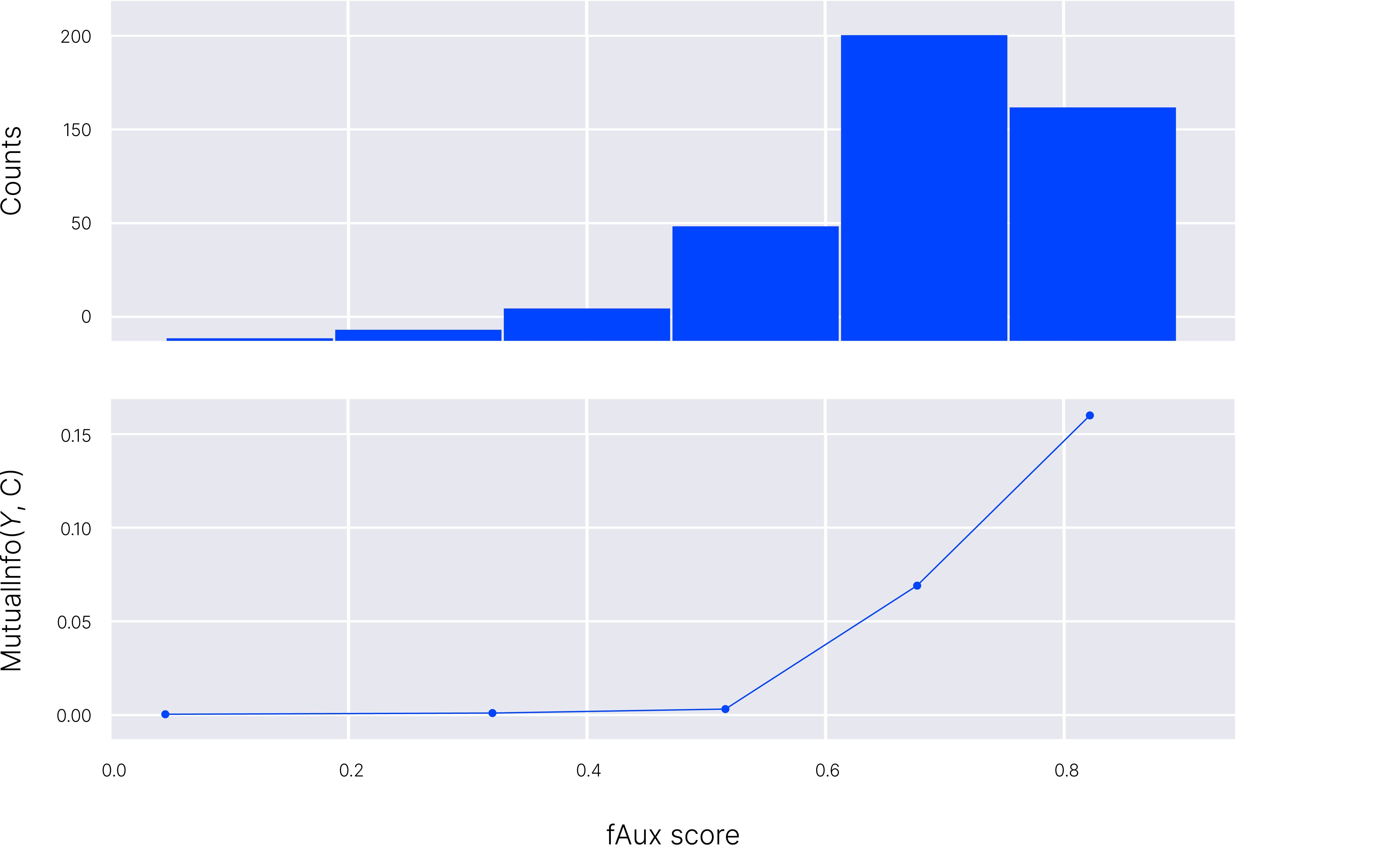
Figure 11: Comparing fAux and independence.
Another, practical question to ask is whether or not the fAux score can distinguish between fair and unfair models. Unlike before, we might not be able to control the bias of the dataset, but, we can still control the models we test! In particular, we expect that training algorithms with stronger regularization for fairness should produce models that are more fair. To this end, we use adversarial training to learn fair models, with increasingly strong regularization. Below, we plot a box diagram to show how the distribution of fAux scores changes as we increase model fairness. We see that the unfair models have a higher average fAux score than the fair models. Success!
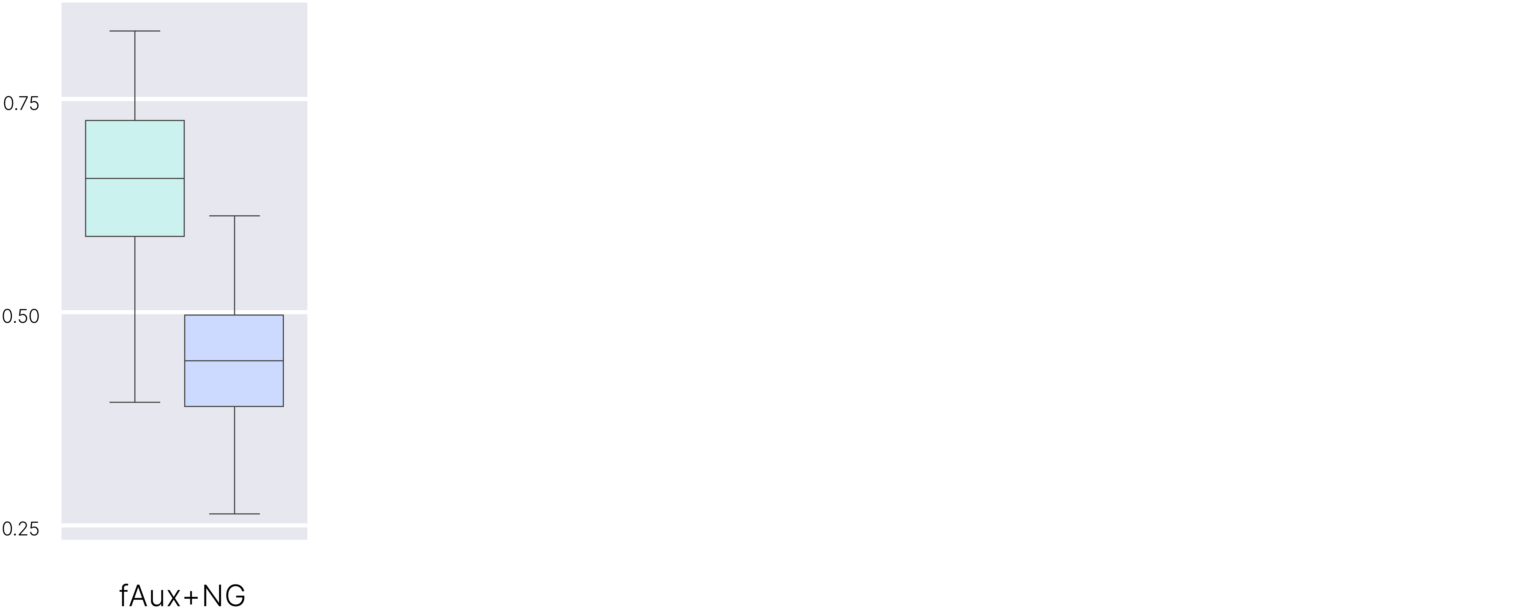
Figure 12: As we make models more fair, we see that the distribution of fAux score shifts downwards.
Thus the average fAux score can distinguish between fair and unfair models.
Finally, an additional advantage of fAux is that it can be used to provide explanations for discriminatory predictions. Let us consider a prediction made by a model that was flagged as discriminatory by fAux. Below we plot a visualization of the prediction. Each of the points corresponds to a feature used by the model in making the decision. The x-axis shows the impact the feature had on the target model’s decisions: more positive means the feature contributed to a positive outcome, more negative means the feature was used to support a negative outcome. The y-axis shows the impact the feature has on the auxiliary model’s decisions. Here, more positive means the feature supports membership in the privileged group, where as more negative means the feature supports membership in a disadvantaged group. The red box is a danger zone: if a feature falls within this box, it is potentially evidence the model provided a negative outcome to an individual based on being in a disadvantaged group. We see that, for this example, the dangerous features – marital status and occupation – are both captured by fAux.
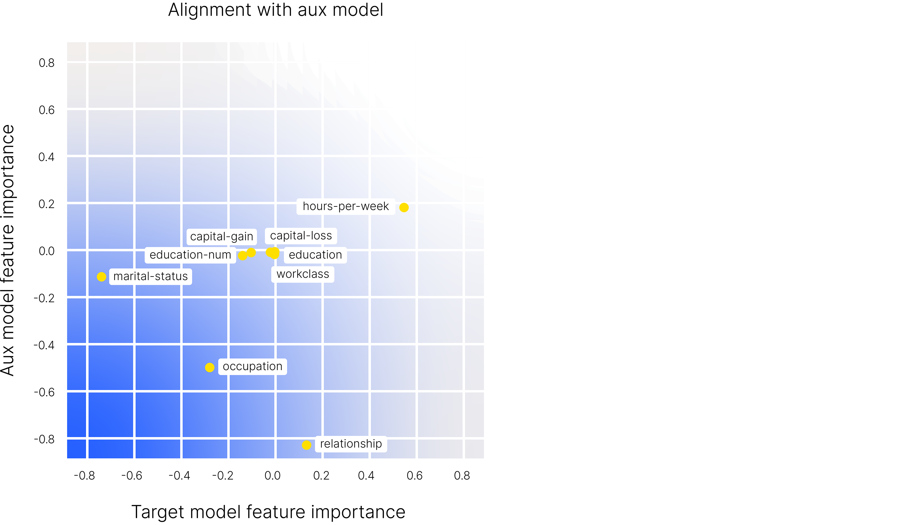
Figure 13: Disecting problematic predictions with fAux. The red box is a ”danger zone.” Features
inside this box are potentially being used to discriminate.
These explanations are potentially useful to model developers, as it provides a tool for debugging both the model and the dataset. Based on the previous analysis, we can see that features such as occupation and marital status are dangerous. What happens if we remove them from the dataset? This is analyzed in the figure below. Here, the red line shows the actual score predicted by the model, which falls short of the correct prediction, shown in green. The blue bars correspond to the Shapley values of the corresponding features, which, heuristically, show the impact of removing that feature on the model’s classification. You’ll note that removing these features from the dataset results in the model making the correct prediction. This is actionable feedback developers can use to ensure their models are safe.
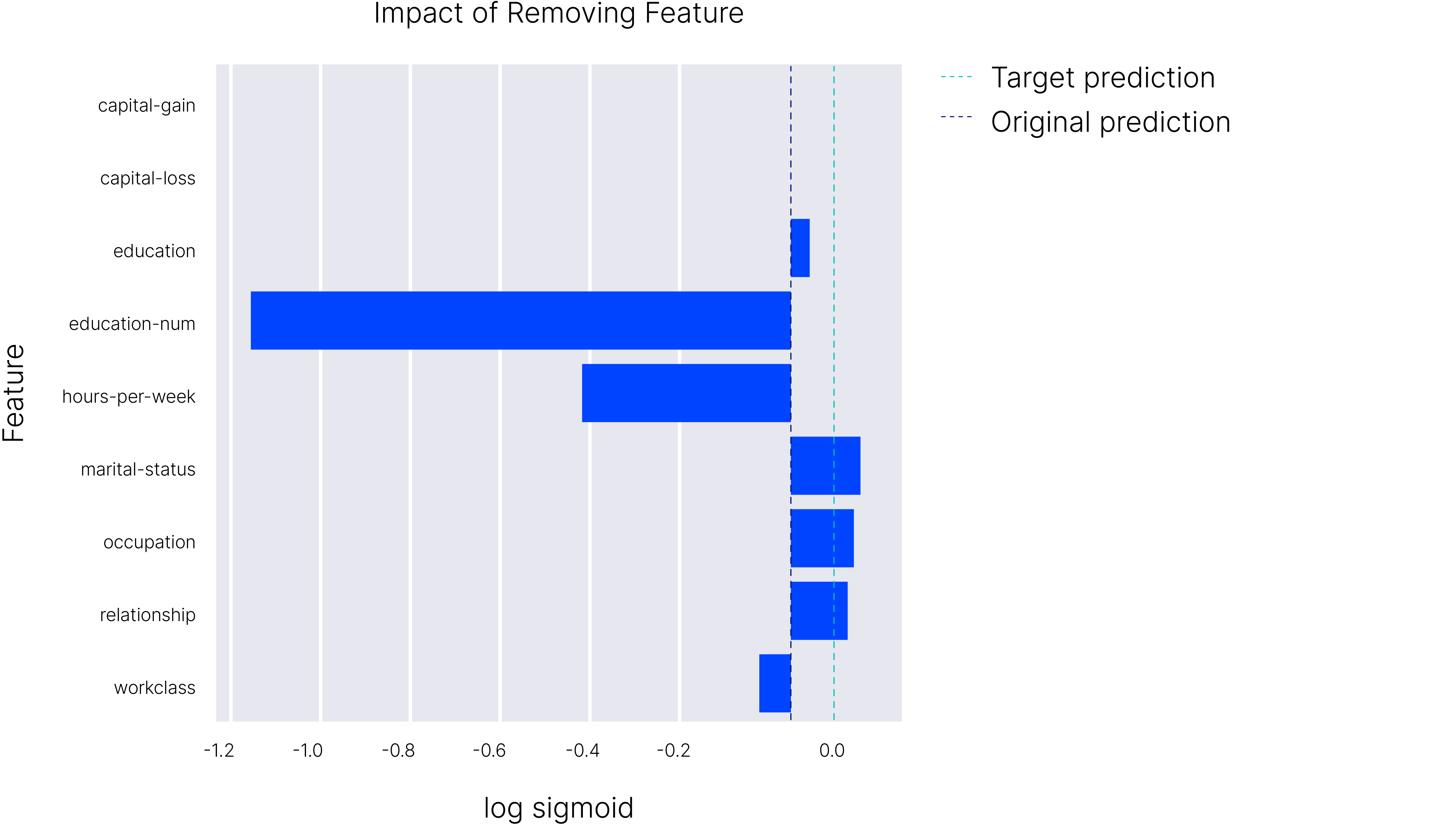
Figure 14: fAux can be used to produce explanations for discriminatory predictions. We see that the
variables ’marital-status,’ ’occupation,’ and ’relationship’ are being used to inform the discriminatory
prediction. Removing these features from the dataset would lead to classifiers that are more fair.
Conclusion
We return to our starting question: when is a model “good?” While this is a subject of active research, we’ve outlined a way that lets us test when models are bad with high precision. In particular, our technique offers a means to test for discriminatory predictions with low model overhead. To verify this, we’ve also introduced a novel framework for adding synthetic patterns of bias into datasets.
There are many ways to extend this work. The flexibility of our test means its possible to test for more than just historical bias. In the future we may consider studying other sources of bias, both demographic and temporal. Moreover, one can consider our test a specific sort of adversarial attack, in which we are generating perturbations in a certain “fair” subspace. It’s thus possible to use formal methods to provide more rigorous certifications of fairness.
While research is ongoing, we hope the work presented can help the community to debug their existing models, and reduce the risk of taking AI outside of the lab.
References
[1] Kunpeng Li, Ziyan Wu, Kuan-Chuan Peng, Jan Ernst, and Yun Fu. Tell me where to look: Guided attention inference network. CoRR, abs/1802.10171, 2018.
[2] Schrasing Tong and Lalana Kagal. Investigating bias in image classification using model explanations. CoRR, abs/2012.05463, 2020.
3] Sahil Verma and Julia Sass Rubin. Fairness definitions explained. 2018 IEEE/ACM International Workshop on Software Fairness (FairWare), pages 1–7, 2018.
[4] Cynthia Dwork, Moritz Hardt, Toniann Pitassi, Omer Reingold, and Richard Zemel. Fairness through awareness. In Proceedings of the 3rd innovations in theoretical computer science conference, pages 214–226, 2012.
[5] Lu Zhang, Yongkai Wu, and Xintao Wu. Achieving non-discrimination in data release. Proceedings of the 23rd ACM SIGKDD International Conference on Knowledge Discovery and Data Mining, 2017.