Adversarial Robustness with AdverTorch Black-box Estimators

We have previously introduced AdverTorch, a toolbox for adversarial robustness research. As part of our initiative at RBC Borealis to create a platform for model validation, we have been building other packages built on top of Advertorch to validate the robustness of different machine learning models and to create visuals to make it easy for developers to interpret the results. 

This tutorial will go through how Advertorch can be used to assess the robustness of any given ML model using the newly added blackbox estimator module in Advertorch. These estimators allow you to use the toolbox for any type of model regardless of the deep learning framework used to develop them in the first place.

Overall the tutorial will cover the following;  

Definition of Adversarial Robustness

In our model validation framework, we broke down every validation scheme into four components;

We have previously covered our approach to adversarial robustness in a previous blog post. At a high level, we are interested in helping model developers and validators find out whether a tiny nudge (of size epsilon) to an input data point X can completely change a prediction made by the original model.

Having defined our statement, we also construct a neighbourhood which encapsulates our input domain with any additional constraints we might want to impose such as different normalizations and valid input checks. Finally, we use a solver to see if any failure examples can be found. If so, we return them to the user as examples of having failed this adversarial robustness test. In the following sections, we will be constructing each of these components.

An adversarially robust model is such that it does not change its original prediction for a given epsilon size. An example of this is shown in figure 1.

​Figure 1: A simple comparison of a robust model and a non robust model. After applying a small perturbation to Feature B and Feature D, the prediction of the robust model stays the same whereas the prediction changes for the non-robust model.

Building a Blackbox Model using AdverTorch

Dataset and Model

Before we can use the blackbox estimator wrapper, we need to build a model. For this tutorial, we will be using an XGBoost classifier on the breast cancer dataset which is conveniently available through sklearn. It is a classic dataset for a binary classification task. The features describe various measurements of the cell nuclei from a digitized image of a breast scan, and the output indicates whether the mass is malignant or benign. The dataset is relatively small, with only 569 samples and 30 features, but it is sufficient for this tutorial. Furthermore, the dataset is ideal for this tutorial since all the features are continuous variables. Features with categorical variables are ignored during the adversarial attack since these cannot be perturbed.

import numpy as np
from sklearn.datasets import load_breast_cancer
from sklearn.model_selection import train_test_split
from sklearn.metrics import accuracy_score
from xgboost import XGBClassifier

dataset = load_breast_cancer()
X, y = dataset.data, dataset.target

X_train, X_test, y_train, y_test = train_test_split(X, y, test_size=0.2)
tree_model = XGBClassifier(n_estimators=50)
tree_model.fit(X_train, y_train)
print("Accuracy: ", accuracy_score(tree_model.predict(X_test), y_test))

Blackbox Estimator

Now we will use the blackbox gradient estimator from AdverTorch. These estimators are built as wrappers around the original models. As the name suggests, the estimator allows us to perform blackbox attacks where we might not have access to the gradients of the models or where the model simply does not have gradients (such as tree-based models). All that is needed to construct a blackbox estimator is the predict function of the model, which returns the class probabilities and an activation function. We will be using the predict_proba function of the XGBoost model. The loss function we’ll be using in Section 3.3 actually requires the log of these probabilities, and so we append an extra function to the model.

Note that one significant disadvantage of this approach is that it is computationally heavy. While iteratively searching for adversarial examples, we will need to perform gradient estimation calculations repeatedly. Moreover, the search will likely take longer since the estimated gradients will not be as accurate as they would be in the case of a white box test.

from advertorch.attacks.blackbox import FDWrapper
import torch.nn as nn

class LambdaLayer(nn.Module):
    def __init__(self, lambd):
        super(LambdaLayer, self).__init__()
        self.lambd = lambd
    def forward(self, x):
        return self.lambd(x)

activation = LambdaLayer(lambda x: torch.log(x))
predict_fcn = lambda x: torch.from_numpy(tree_model.predict_proba(x))
pred_fcn = FDWrapper(func=predict_fcn, fd_eta=5.0)
bb_estimator = nn.Sequential(pred_fcn, activation)

Accuracy: 0.9649122807017544

Adversarial Robustness Validation Using AdverTorch

Statement

As mentioned previously, we are assessing the robustness for a classification task. Our decision statement in this case is to find whether there exists x ′∈ Ball(x, ϵ) such that F(x ′ )̸=y.

To this end, we check whether a given adversarial example, x ′ , is inside our neighbourhood Ball(x, ϵ), and that F(x ′ )! = y. The given adversarial example passes our decision statement if both conditions are met.

class RobustClassification:
    """For all inputs in a given neighbourhood, check if the model predicts the
    same class (according to argmax)"""
    def __init__(self, neighbourhood, model):
        self.neighbourhood = neighbourhood
        self.model = model

    def pred(self, x):
        with torch.no_grad():
            y = self.model(x).argmax(-1)
        return y

    def eval_input(self, X, Xprime, epsilon):
        return self.neighbourhood(Xprime, X) <= epsilon

       def eval_output(self, Y, Yprime):
            return Y != Yprime
   
       def eval_counterexample(self, X, Xprime, epsilon):
           valid_input = self.eval_input(X, Xprime, epsilon)
           Y, Yprime = self.pred(X), self.pred(Xprime)
           invalid_output = self.eval_output(Y, Yprime)
           return valid_input & invalid_output

Neighbourhood

Now we construct the neighborhood, which allows us to check whether a given adversarial example lies within the constraints we would like to impose. For this tutorial, we will be using a scaled L-inf norm constraint. For each counter-example, we will check if the following condition holds;

Since we’re using an infinity norm, the ϵ ball is, in reality, a rectangle. To ensure that the adversarial example lies within, we also need to scale our features, i.e. normalize the data points or equivalently scale the ϵ according to the feature range. However, we need first to construct a dictionary containing all the necessary information for each of the features, such as the valid input range, scale, feature name, and feature type (“REAL”, “BIN” or “INT”). There is also a flag to tell the solver to ignore a given feature. The ignore flag will allow us to select the features we want to perturb and ignore those we cannot perturb. The valid input range will enable us to build a conditional mask to enforce the validity of the generated adversarial examples. Features outside of the valid range are masked and thus not perturbed.

data_config = []

for i in range(len(dataset.feature_names)):
    data_config.append(
        {
            "Feature": dataset.feature_names[i],
            "Feature_type": "REAL",
            "ignore": False,
            "ranges": [min(dataset.data[i]), max(dataset.data[i])],
            "scales": max(dataset.data[i]) - min(dataset.data[i]),
         }
    )

import torch
from typing import Tuple, List, Dict
from advertorch.utils import clamp as batch_clamp

class ScaledLinfNeighbourhood(nn.Module):
    def __init__( self, config: List[Dict]):
        nn.Module.__init__(self)
        self.set_scales(config)
   
    def __call__(self, x1: torch.FloatTensor, x2: torch.FloatTensor) -> torch.
  ↪→FloatTensor:
        z1, z2 = self.transform(x1), self.transform(x2)
        return (abs(z1 - z2)).max(-1)[0]

    def set_scales(self, config: List[Dict]):
        n_dim = len(config)
        mins, maxs, intmask, ignore = (torch.zeros(n_dim) for _ in range(4))
        scales = torch.ones(n_dim)
       
        for i, feature in enumerate(config):
            if not feature["ignore"]:
                mins[i], maxs[i] = feature["ranges"]
                scales[i] = feature["scales"]

            intmask[i] = feature["Feature_type"] in ["BIN", "INT"]
            ignore[i] = feature["ignore"]
        self.register_buffer("mins", mins)
        self.register_buffer("maxs", maxs)
        self.register_buffer("scales", scales)
        self.register_buffer("intmask", intmask.bool())
        self.register_buffer("ignore", ignore.bool())

        def bounds(self, x: torch.FloatTensor, eps: torch.FloatTensor):
            outlier_mask = (x < self.mins) | (x > self.maxs)
            mask = outlier_mask | self.ignore
            eps_max = torch.min(x + eps[:, None] * self.scales, self.maxs)
            eps_min = torch.max(x - eps[:, None] * self.scales, self.mins)
            bmin = mask * x + ~mask * eps_min - 1e-9
            bmax = mask * x + ~mask * eps_max + 1e-9
           
            return bmin, bmax

        def transform(self, x: torch.FloatTensor) -> torch.FloatTensor:
            return (x - self.mins) / self.scales

        def inverse_transform(self, x: torch.FloatTensor) -> torch.FloatTensor:
            return x * self.scales + self.mins

        def project(self, x: torch.FloatTensor, bounds) -> torch.FloatTensor:
            # Clamp to Linf Ball
            bmin, bmax = bounds
            batch_clamp(x, bmin, bmax)
           
            # Fix integers
            f, c = torch.floor(x), torch.ceil(x)
            floor_check = (f >= bmin) & (f <= bmax)
            rounded = torch.where(floor_check, f, c).float()

            x = torch.where(self.intmask.bool(), rounded, x)

            return x
           

Solver

We use Projected Gradient Descent (PGD) to search for points in the input space which violate a statement of behavior. These points are obtained from the original dataset using small perturbations and are found by optimizing a surrogate loss corresponding to the statement. We use the perturb_iterative function which is found in advertorch. It’s a shared method for iterative attacks, including LinfPGD which is what we will be using. We chose PGD for its simplicity; the same idea could be extended to other solvers.

The solver uses the neighbourhood to get the boundaries of the search space and to apply the necessary transformations as needed. generate_counterexamples has three important parameters that significantly affects the advarserial example search.

linf_eps: epsilon size
linf_eps_iter: epsilon step-size per iteration
linf_nb_iter: number of iterations

from advertorch.attacks.iterative_projected_gradient import perturb_iterative

class LinfPGDSolver:
    def __init__(self, statement, loss = nn.NLLLoss(reduction="sum")):
        self.statement = statement
        self.loss = loss
        self.model = self.build_model()

    def build_model(self): 
        decoder = LambdaLayer(lambda x: self.decode(x))
        return nn.Sequential(decoder, self.statement.model)

    @property
    def neighbourhood(self):
        return self.statement.neighbourhood

    def encode(self, x: torch.FloatTensor):
        return self.neighbourhood.transform(x)

    def decode(self, x: torch.FloatTensor):
        return self.neighbourhood.inverse_transform(x)

    def _get_clip_bounds(self, X: torch.FloatTensor, eps: torch.FloatTensor) ->␣
  ↪→Tuple[torch.FloatTensor, torch.FloatTensor]:
        bmin, bmax = self.neighbourhood.bounds(X, eps)
        bmin, bmax = self.encode(bmin), self.encode(bmax)
        return bmin, bmax

    def generate_counterexamples(
        self, X: torch.FloatTensor, Y: torch.Tensor, linf_eps = 0.2,␣
   ↪→linf_eps_iter = 0.0625, linf_nb_iter = 500
    ) -> torch.FloatTensor:
        n_batch, _ = X.shape
        linf_eps = linf_eps * X.new_ones((n_batch,))
        bmin, bmax = self._get_clip_bounds(X, linf_eps)
        Xe = self.encode(X)
        adv = perturb_iterative(
            xvar=Xe,
            yvar=Y,
            predict=self.model,
            nb_iter=linf_nb_iter,
            eps=linf_eps,
            eps_iter=linf_eps_iter,
            loss_fn=self.loss,
            minimize=False,
            clip_min=bmin,
            clip_max=bmax,
        ).detach()

        adv, bmin, bmax = self.decode(adv), self.decode(bmin),self.decode(bmax)
        adv = self.neighbourhood.project(adv, (bmin, bmax))
       
        return adv

Search for Adversarial Examples

Finally, we are ready to perform a binary search to find the best adversarial examples, i.e counterexamples that satisfy all our constraints with the slightest perturbation possible. We search for the best adversarial examples for a fixed number of iterations. The number of iterations in our binary search algorithm, the number of iterations that we use for the solver, and the number of samples we use for gradient estimators all contribute to the overall complexity of our test. When setting these values, readers should be mindful to ensure the adversarial examples are found within a reasonable time frame. 

neighbourhood = ScaledLinfNeighbourhood(data_config)
statement = RobustClassification(neighbourhood, bb_estimator)
solver = LinfPGDSolver(statement=statement)

def binary_search_over_param(
    X: torch.Tensor,
    Y: torch.Tensor,
    statement,
    solver,
    init_val: float = 0.1, 
    min_val: float = 0.0,
    max_val: float = 1.0,
    max_bin_iter: int = 5,
    seed: int = 0,
    params_for_solver: dict = {},
) -> Tuple[torch.FloatTensor, torch.FloatTensor]:
    torch.manual_seed(seed)
    n_batch, _ = X.shape
    cur_min = X.new_full((n_batch,), min_val)
    cur_max = X.new_full((n_batch,), max_val)
    cur_val = X.new_full((n_batch,), init_val)
    best_adv = torch.zeros_like(X)
    solver_dict = dict(params_for_solver)
    for i in range(max_bin_iter):
        solver_dict['linf_eps'] = cur_val
        adv = solver.generate_counterexamples(X, Y, **solver_dict)
        violations = statement.eval_counterexample(X, adv, cur_val)
        best_adv[violations] = adv[violations]
        cur_min = torch.where(violations, cur_min, cur_val)
        cur_max = torch.where(violations, cur_val, cur_max)
        cur_val = (cur_min + cur_max) / 2
    return best_adv, cur_max

best_adv, best_eps = binary_search_over_param(
    X=torch.Tensor(X_test),
    Y=torch.LongTensor(y_test),
    statement=statement,
    solver=solver,
    max_bin_iter=10,
    seed=0,
    params_for_solver = {
        'linf_eps_iter':0.0625,
        'linf_nb_iter':100
    }
)

Interpreting the Results

Now that we have our adversarial examples, we would like to evaluate them. We show a few plots which are useful in understanding how robust a given model is. However, it is essential to note that robustness is not easily quantifiable. Therefore, we do not provide any concrete metric to measure robustness. We instead attempt to give some insight which may be useful to the reader. The plots can be used in isolation, but they are much more insightful when comparing two models or throughout the model development phase.

Flip Rate vs Epsilon Size

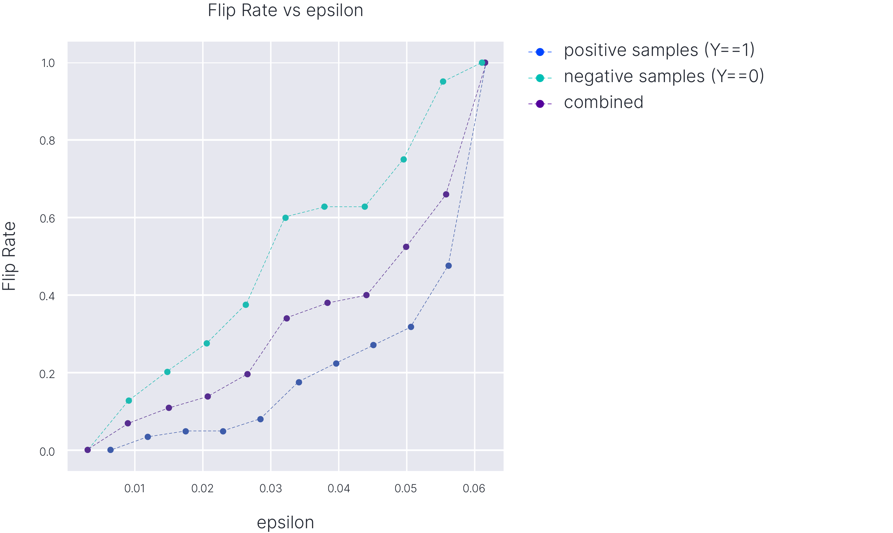
Epsilon size is the amount of perturbation required to generate a counterexample. The mean epsilon size is the average of all epsilon sizes found during the adversarial example search. The higher the mean epsilon size, the higher the robustness. This value is best interpreted in comparison to competing models.

Flip rate is the fraction of the test dataset for which we could find adversarial examples, i.e., flip the label from 0 to 1 or from 1 to 0. It is helpful to see how the flip rate changes as the size of the epsilon ball changes. It is also beneficial to see how samples with different labels perform. In this toy example, we see that samples from positive samples (y=1) are slightly less robust compared to the negative samples (y=0). This may be important depending on the application and the metric being used for the model’s performance.

import matplotlib.pyplot as plt
# Compute mean epsilon
y_prob = tree_model.predict_proba(X_test)[:, 1]
y_prob_best_adv = tree_model.predict_proba(best_adv)[:, 1]
threshold = 0.5

idx = best_eps != 1.0
print(f'Flip Rate is {sum(idx)/len(best_eps)}%.')
print(f'Mean epsilon size is {best_eps[idx].mean()}.')

def cumulative_dist_plot(x, bins, ax, **kwargs):
values, base = np.histogram(x, bins=bins)
cumulative = np.insert(np.cumsum(values), 0, 0.0)
cumulative = cumulative / cumulative[-1]
return ax.errorbar(base, cumulative, **kwargs)

plt.style.use('ggplot')
fig, ax = plt.subplots(1, 1, figsize=(8,8))
plot_config = {'bins':10, 'ax':ax, 'marker':'o', 'linestyle':'--'}
cumulative_dist_plot(best_eps[(torch.Tensor(y_test)==1) & idx].cpu().numpy(),␣
↪→label='positive samples (Y==1)', **plot_config)
cumulative_dist_plot(best_eps[(torch.Tensor(y_test)==0) & idx].cpu().numpy(),␣
↪→label='negative samples (Y==0)', **plot_config)
cumulative_dist_plot(best_eps[idx].cpu().numpy(), label='combined',␣
↪→**plot_config)

plt.legend()
plt.xlabel('epsilon', fontsize=20)
plt.ylabel('Flip Rate', fontsize=20)
plt.title('Flip Rate vs epsilon', fontsize=20)
plt.show()

Flip Rate is 0.9298245906829834%.
Mean epsilon size is 0.048476193100214005

Initial vs Perturbed Score

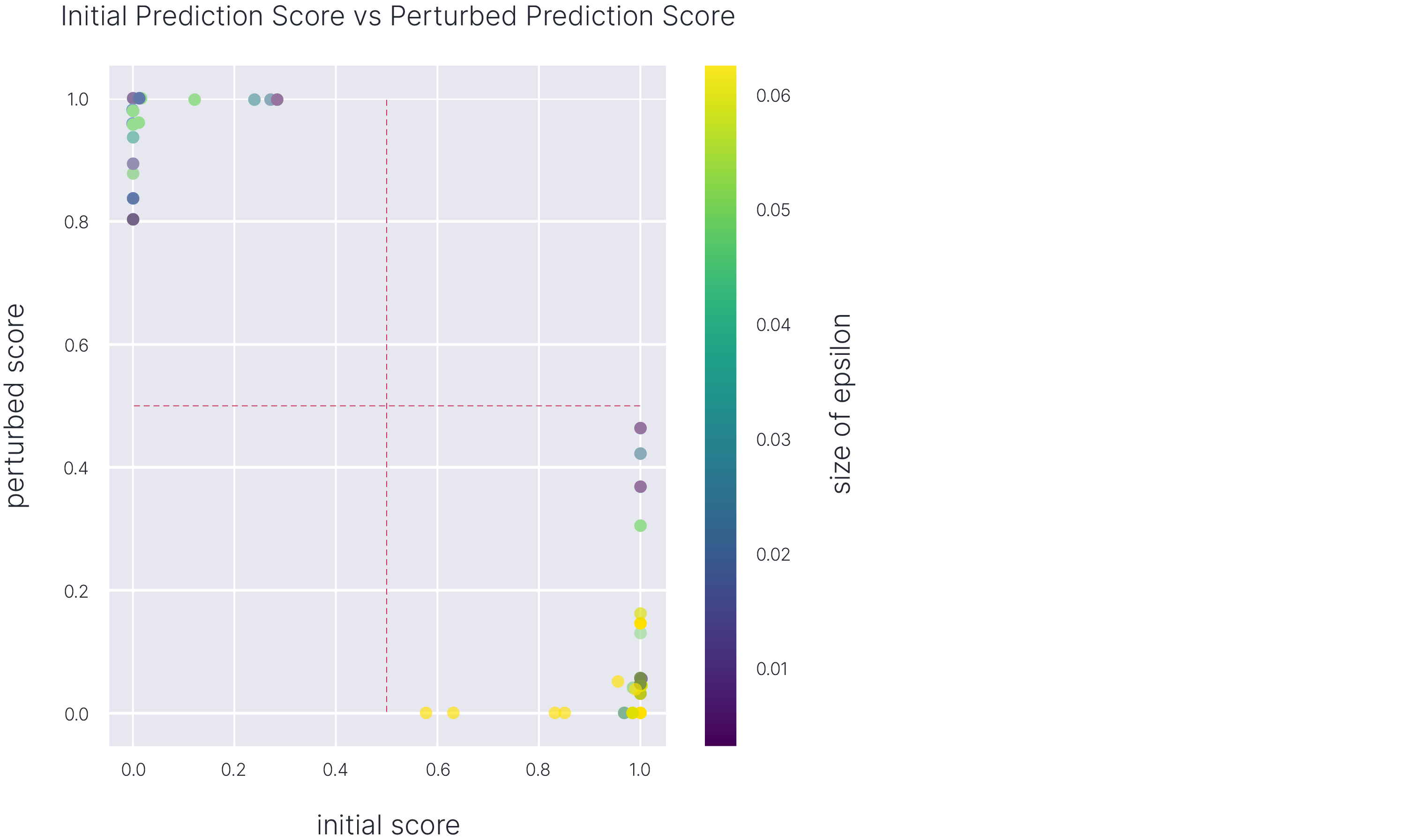
This plot shows how successful the adversarial search is in changing the model’s predictions. Here, we generate a color-coded scatter plot, where each point corresponds to a sample. The point coordinates tell us the model prediction for the original sample and the corresponding adversarial example.

The points in the upper left corner and lower right corner are of particular interest to the users. These are the points that were originally predicted with a strong probability score and are now being labeled with the opposite label with a strong probability score. The color of the points is also crucial as it indicates the epsilon size. The points with smaller epsilon sizes are more concerning than others as it means these points are susceptible to perturbations.

fig, ax = plt.subplots(1, 1, figsize=(8,8))

sc = ax.scatter(x=y_prob[idx],
        y=y_prob_best_adv[idx],
        c=best_eps[idx],
        alpha=0.5)

cbar = plt.colorbar(sc)
cbar.set_label('size of epsilon', fontsize=12)
plt.xlabel('initial score', fontsize=20)
plt.ylabel('perturbed score', fontsize=20)

plt.hlines(0.5, 0, 1, linestyles="--")
_ = plt.vlines(0.5, 0, 1, linestyles="--")
plt.title('Initial Prediction Score vs Perturbed Prediction Score', fontsize=20)

Out-of-Distribution Check

Lastly, we investigate whether the counter-examples found in the attack align with the original dataset. If there is a significant difference in distribution from the original dataset, the adversarial examples might not be of much concern. They can be detected as outliers in production and ignored. We will use Isolation Forest for this tutorial to see if any of our adversarial examples are detected as an outlier.

from sklearn.ensemble import IsolationForest

clf = IsolationForest().fit(X_test)
print(f'{sum(clf.predict(best_adv) == 1)} samples detected as outliers')

0 samples detected as outliers

In addition, we will use the Proxy-A Distance (PAD) as a metric to measure how the adversarial example distribution shifts from original data points. We train a new model to distinguish adversarial examples from the original dataset. We combine the test dataset with the adversarial examples and create output labels where the samples from the original dataset are marked as 0, and the adversarial examples are marked as 1. As a model, we select XGBoost classifier to distinguish the two. Finally, we get the MAE score on our test set and compute the PAD measure as 1−2 ∗MAE. The lower the PAD score, the closer the two datasets are.

from sklearn.metrics import mean_absolute_error

x_adv = best_adv[idx]
y_prob_threshold = 0.5

# Train auxiliary model to classify adversarial examples.
# Combine the datasets
x_comb = np.r_[x_adv, X_test]
y_comb = np.r_[np.ones(x_adv.shape[0]), np.zeros(X_test.shape[0])]
x_comb_train, x_comb_test, y_comb_train, y_comb_test = train_test_split(x_comb,␣
↪→y_comb, train_size=0.7)
# Train a simple XGBoost classifier
model = XGBClassifier(n_estimators=5).fit(x_comb_train, y_comb_train)

# Compute MAE on test set
y_pred = [1-prob[0] for prob in model.predict_proba(x_comb_test)]
mae = mean_absolute_error(np.array(y_pred), y_comb_test)

# Compute Proxy-A distance
proxy_a_score = 1 - 2*mae

print(f'Proxy-A distance: {proxy_a_score}')

Proxy-A distance: 0.760538379351298

Final Remarks

This tutorial is meant to demonstrate an approach to validation using four main building blocks (statements, neighbourhoods, solvers and models) and also provide some techniques we found to be useful when communicating adversarial robustness results. A jupyter notebook version of this tutorial can be found on Github.