
This article describes a system called Aiden, developed jointly by RBC Capital Markets and RBC Borealis. At a high level, Aiden aims to solve the following problem: a customer indicates that they wish to buy or sell a certain number of units of an asset and it is the broker’s responsibility to execute this order within a specified time window, seeking prices that minimize loss relative to a specified benchmark. For simplicity of exposition this article is restricted to the former case (buy orders).
This execution problem sounds straightforward but there are several complications. A naive approach might be to wait until the price seems “low enough” and then buy all the shares at once. Putting aside the question of how to define “low enough”, this method has a huge drawback. Executing a large order all at once creates a great deal of demand and the effect of this is to increase the price (market impact). Unfortunately, this action has an undesirable effect on the final price achieved. Consequently, it could be more sensible to buy the shares gradually through the specified time period. But how many should the broker buy, and when?
To the savvy machine learning researcher, it will be obvious that this problem lends itself to a reinforcement learning formulation. The execution algorithm must make a series of sequential decisions about how many shares to buy at each time step and receives rewards in the form of low execution prices.
The structure of the rest of this article is as follows. First, we describe the order execution problem in more detail. This will necessitate a discussion of how modern financial markets work in practice and the limit order book. Then we provide a brief review of reinforcement learning and describe how it maps to this problem. Finally, we describe the practical details of the Aiden system.
Limit order markets
Contemporary financial markets such as the TSX/NYSE/NASDAQ are limit order markets. This means that traders who wish to purchase shares can specify not only the volume they wish to purchase, but also the maximum price (limit) that they are prepared to pay. More formally, a limit order can be specified by the tuple $\{\tau, p, n\}$ where $\tau\in\{0,1\}$ specifies whether this is a buy or sell order, $p$ is the specified price limit, and $n$ is the maximum number of shares to be traded. The possible prices of the shares in the order book are discrete, and the smallest difference allowable between them is a tick.
The limit order book consists of the set of all current limit orders. It can be visualized as two histograms (figure 1). The first consists of the volume of the buy orders at each discrete price level and the second consists of volumes of the sell orders. The highest buy order is known as the current bid price and the lowest sell order is known as the current ask price. The difference between the two is known as the bid-ask spread and the average of the two is known as the mid-price.
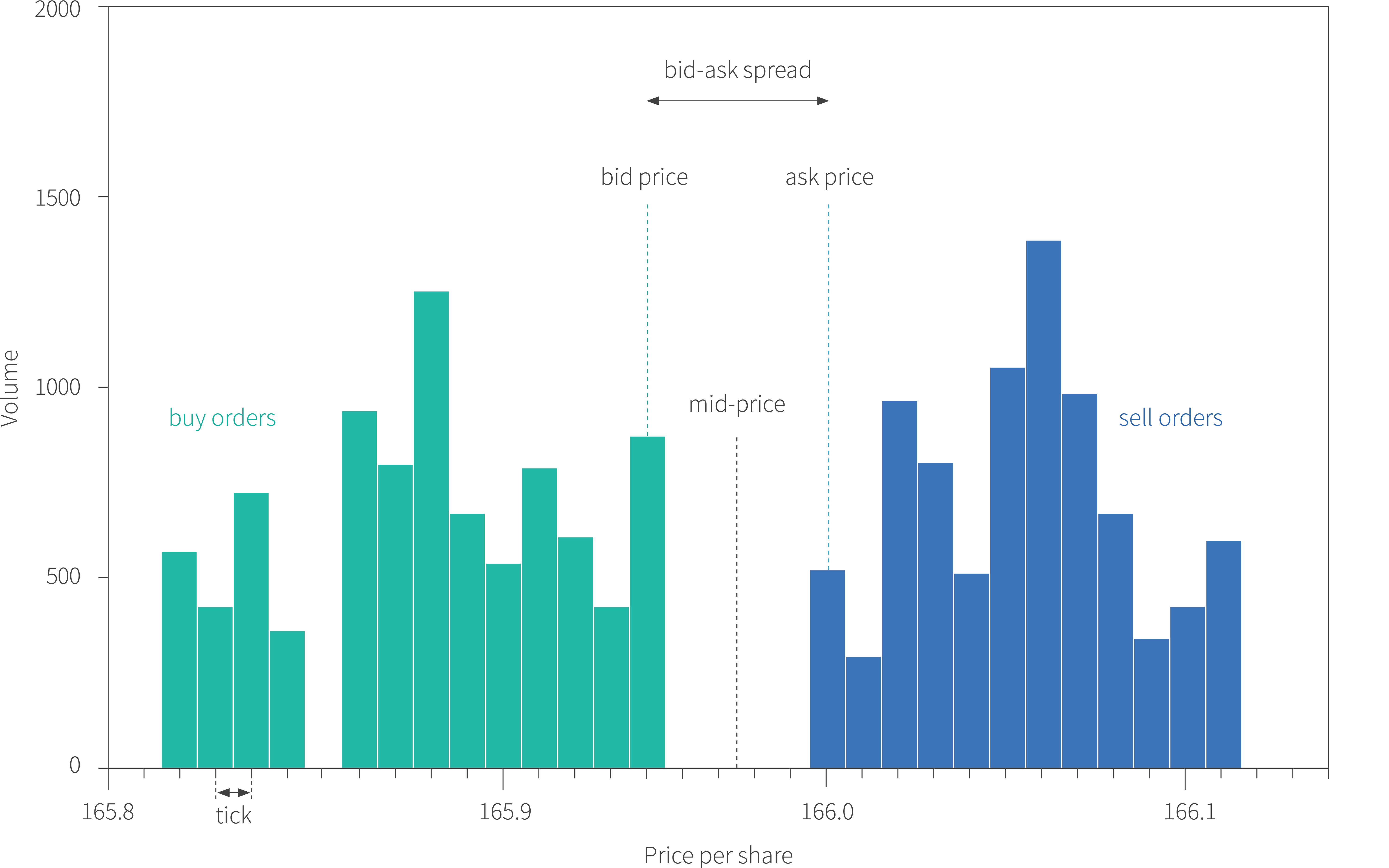
Figure 1. Limit order book. The limit order book contains information about current buy and sell orders at each discrete price level or tick. The buy orders are indicated by green bars and the sell orders are indicated by blue bars. In each case, the horizontal position of the bar indicates the price and the height of the bar represents the volume. In a single market scenario, the ranges of the two histograms are always non-overlapping; if they were not then the buy and sell prices would match and a transaction would occur. The highest price offered to buy shares is known as the bid price and the lowest price offered to sell is known as the ask price. The distance between these prices (and hence between the histograms) is known as the bid-ask spread. The average of these two prices is termed the mid-price and can be thought of as the current price of the asset.
Limit orders
When a trader enters a buy limit order that is at or above the current ask price, the order will receive executions. The first trades will occur at the current ask price, but if the volume of the buy order exceeds the volume available at that price, the order will continue at the next price level. This process occurs until either the entire order has been fulfilled, or it reaches the specified limit. In this case, there are insufficient shares available for sale at or below this limit and so the order is only partially filled. Hence, the overall effect of placing a limit order is that the price is guaranteed to be within the specified limit, but the volume is not.
Any remaining unfulfilled part of the order is then added to the buy side of the limit order book and remains there until it is either (i) matched by a new sell-side order (ii) its time limit expires or (iii) it is removed by the trader. Orders are typically matched based on a first-in / first-out basis for most trading venues; in this instance, any order placed below the current ask price will be placed last in the queue for that particular price level. A worked example of a limit order is given in figure 2.
Figure 2. Limit order example. Starting with the situation in figure 1, a buy order is placed for 1750 shares with a limit of 166.01, meaning that this is the maximum price the trader is prepared to pay for them. This order is first matched with the lowest possible price and 500 shares are bought at a price of 166.00 (represented by left-most pale blue bar). This leaves 1250 unfulfilled units in the buy order. The next lowest price (166.01) is also within the limit and so we also purchase all of the 250 shares at this level (represented by right-most pale blue bar). This leaves 1000 unfulfilled units in the buy order. Unfortunately, the next price on the sell side is above the specified limit and so no further transactions occur at this time. The remaining order for 1000 shares is entered into the limit order book (rightmost green bar). Note that the effect of this is that both the bid and ask prices increase and hence so does the mid-price. Placing this aggressive order increases the effective price of the asset.
Market orders
In addition to limit orders it is possible to place a market order which is specified by the volume $n$ of shares that we wish to buy. Essentially, this means that the trader will buy all $n$ shares now at whatever prices are available on the sell side of the limit order book. So first the trader buys shares at the current ask price. If the volume of the buy order exceeds the volume available at the current ask price, the trader will continue fulfilling the order at the next best price and so on. Effectively, a market order is hence a limit order where the limit is $+\infty$. A worked example of a market order is given in figure 3.
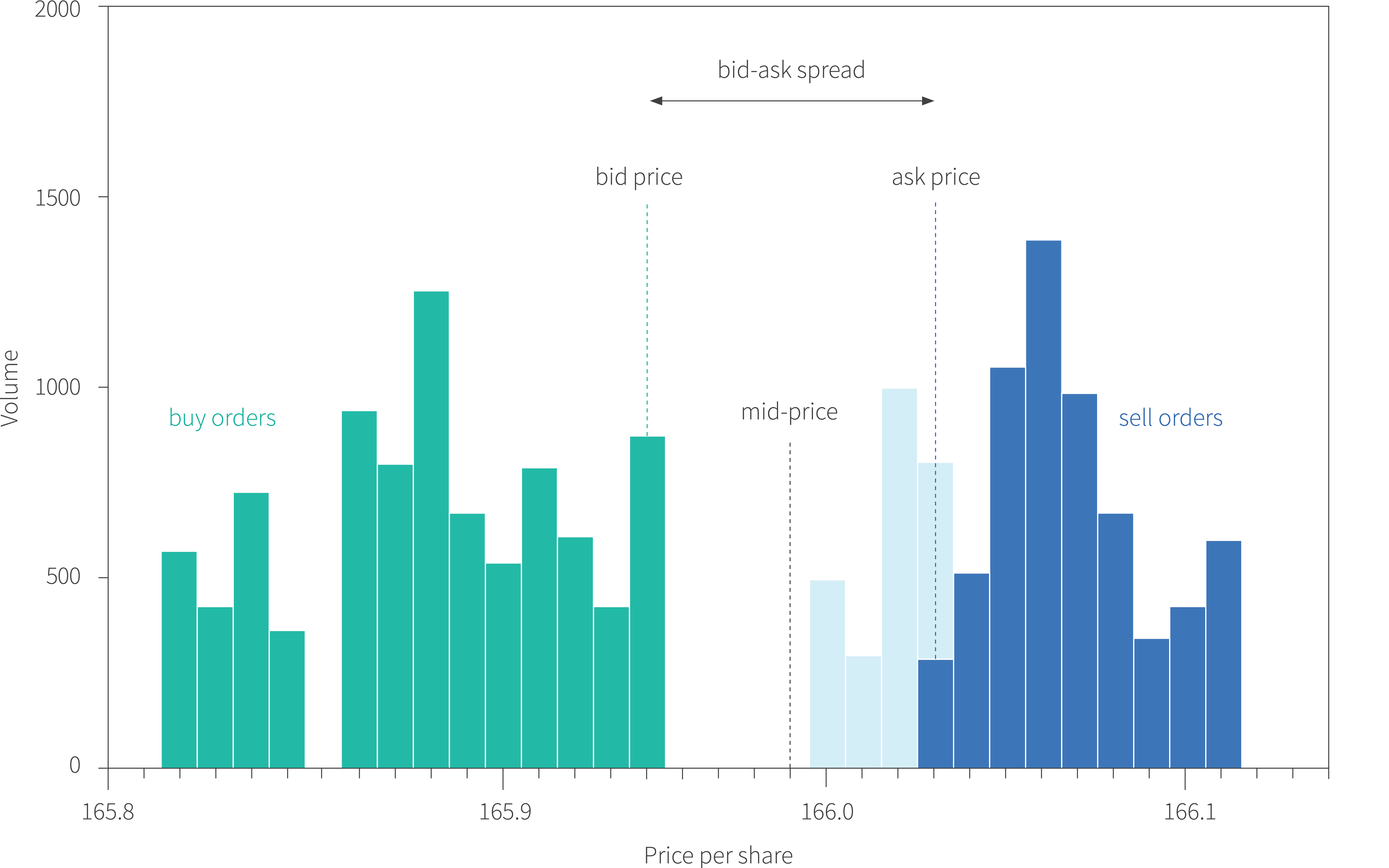
Figure 3. Market order example. Starting with the situation in figure 1, the trader places a market buy order for 2250 shares. To fulfil this order, they first look to the lowest possible sell price of 166.00 and since there are only 500 units for sale at this price, they buy all of them (leftmost pale blue bar). The trader continues in this way, buying all of the units at prices 166.01 and 166.02. The volume for sale at 166.03 is sufficient to fulfil the remaining part of the order and some shares are left for sale at this level which becomes the new ask price. Hence, after a market buy order, the ask price increases, but the bid price remains the same. It follows that the bid-ask spread and the mid-price must both increase. Once more, the demand created by the order causes the effective price to inflate.
Market impact of orders
Notice that for both the limit order and the market order, a large volume affects the current ask price. As the volume at one price level is exhausted the ask price increases to the next level where there is non-zero volume. Hence, by placing a large volume buy order, ceteris paribus, it may have a large impact on the market and the mid-price (a proxy for current stock price) correspondingly increases.
Order execution
Now that limit order book has been explained, let’s return to the problem of order execution. The goal is to buy a known volume $V$ of shares within a given time window $[0,T]$. This is typically referred to as the parent order (or meta order). At each time step $0\leq t < T$ the trader can place a limit order, remove an existing limit order, or place a market order by tranching parts of the meta order into smaller parts (child orders) as to minimize market impact. As the trader reaches the end of the execution timeframe, they can make use of more aggressively priced orders to complete their order, potentially at a higher cost.
Market micro-structure data
How can a trader decide which action to take at each time step? Electronic markets release in real-time the contents of the limit order book and the trader can use this data as a basis for their decisions. Such market micro-structure data comes in two different resolutions which are referred to as level I and level II data respectively. Level I data includes the current bid price and associated volume, the current ask price and associated volume and the price and volume of the last transaction. Level II data includes more details about the contents of the limit order book; for example, it might include the top ten current bid and ask orders and their associated volumes.
It’s clear that this market micro-structure data contains clues about when it might be a good idea to place an order. For example, if the ask-price is decreasing over time, it might be worth using this momentum signal to delay buying shares. Similarly, if there is a lot more volume on the sell side than the buy side of the limit order book then this gives an insight into the current levels of supply and demand and this may similarly affect the decision to execute an order at this time or not. In addition, the time stamp and volume already executed should feed into the decision. If time is running out, the trader needs to place more aggressive orders to fulfil their obligation.
Reinforcement learning
In this section we provide a brief recap of reinforcement learning (RL). RL is concerned with an agent that is interacting with an environment. At each time-step $t$, the state of the environment is captured in a state vector $\mathbf{s}_{t}$. The agent observes this state and chooses an action which is parameterized by the vector $\mathbf{a}_{t}$. Taking an action triggers two events. First the state changes to a new state $\mathbf{s}_{t+1}$ via the stochastic transition function $Pr(\mathbf{s}_{t+1}|\mathbf{s}_{t}, \mathbf{a}_{t})$. Second, a reward $r_{t}$ may be issued to the agent, where this reward depends on the unseen reward function $Pr(r_{t}|\mathbf{s}_{t}, \mathbf{a}_{t})$. The basic RL setup is shown in figure 4.

Figure 4. Reinforcement learning setup. The agent makes a decision which is represented by the action $\mathbf{a}$. This action triggers a change in the environment which is represented by the state $\mathbf{s}$ and results in a scalar reward $r$. These two quantities are used by the agent to choose the next action. The agent must learn to recognize which actions it should choose in which states, so that the total rewards received over time are maximized.
At any time $t’$ the agent might wish to maximize the total sum of future rewards $\sum_{t=t’}^{T}r_{t}$. However, rewards that happen sooner in time are often considered more important, and so instead it maximizes the discounted sum of rewards $\sum_{t=t’}^{T}\gamma^{t-t’}r_{t}$. Here $\gamma\in(0,1]$ controls how the rewards decrease in importance as they stretch into the future. So the goal of reinforcement learning is to learn how to choose actions that maximize the sum of the future discounted rewards.
Reinforcement learning is challenging for a number of reasons ranging from practical considerations and design choices to inherent limitations of the RL framework. First, the agent does not know either the transition function or the reward function and it must either implicitly or explicitly learn these. Second, these functions are stochastic, and so it may take a lot of experience to understand them. Third, the reward for an action may be temporally very distant from the action that caused it. This is known as the temporal credit assignment problem. For example, a win in chess may have been largely due to a brilliant move (action) that was made much earlier in the game, yet is only observed by the reward (winning the game) at the end.
Finally, reinforcement learning algorithms must balance exploration and exploitation. On the one hand, if the agent does not explore the state space and try different actions, it cannot get enough experience to learn a good strategy. On the other, once it has figured out how to receive a respectable reward, it might want to exploit this knowledge rather than explore the other regions of the state-action space. A trade-off between these two tendencies is inherent in any reinforcement learning algorithm.
Types of RL algorithm
Model-based methods try to predict what the next state and/or reward will be (i.e., the transition function and the reward function), so that they can look into the future and make sensible decisions that will ultimately result in high cumulative rewards. In contrast, model-free methods do not build a model of the environment or reward, but just directly map states to actions. Model-free methods can be divided into policy-based methods which directly predict a probability distribution over the possible actions from the state and value-based methods which compute the relative value of every possible state-action pair and hence indirectly specify the best action for any state.
The Aiden system described in this article is a policy-based model-free method and so it aims to take the state $\mathbf{s}_{t}$ and predict a probability distribution $Pr(\mathbf{a}_{t}|\mathbf{s}_{t}, \boldsymbol\theta)$ over which action $\mathbf{a}$ to take. Since the state space is high-dimensional and data is very limited, Aiden approximates this mapping using a neural network, with parameters $\boldsymbol\theta$. The goal of learning is to ensure that these parameters lead to actions that result in high cumulative rewards.
Reinforcement learning for order execution
Hopefully, it is becoming increasingly clear why reinforcement learning is a suitable way to carry out the order execution problem. There is a reward (the average price at which the agent bought the shares), but the agent does not know the extent of this reward until it has completely fulfilled the order. There is a partially observed state which includes the market micro-structure data, the elapsed time, and the remaining volume. Finally, there are a number of actions that can be taken at any time (placing limit orders, removing limit orders, placing market orders). It’s clear that these actions affect the state by changing the configuration of the market and depleting the remaining volume.
In this context the goal of the reinforcement learning algorithm is to learn the policy; for a given observed state (market micro-structure, elapsed time and remaining volume), it must learn to output a probability distribution over the possible actions (types of order). The algorithm draws from this distribution to determine what to do next. This in turn changes the state and so on.
Aiden setup
In this section we describe the main features of the Aiden reinforcement learning setup: the action space, the state and the reward functions. In the subsequent section we discuss the reinforcement learning algorithm itself.
Action
In practice Aiden does not directly select the details of the order that is provided to Aiden, but instead chooses between different high-level actions at each time step that correspond to different levels of aggressiveness as Aiden begins to liquidate the parent order using child orders. These range from crossing the spread (and so immediately executing some of the order) at one end of the spectrum to doing nothing / removing existing orders at the other. These actions form the input to a system that translates them into concrete limit orders.
State
Aiden’s state is currently composed of several hundred market features and self-aware features. The market features comprise of hand-crafted functions that compute quantities of interest from the market micro-structure data. Examples might include measurements of the liquidity, recent price changes, or whether there is an imbalance between the bid and ask volumes. The self-aware features relate to the history of previous actions that Aiden has taken. For example, they might include measurements of how aggressive Aiden has been in recent time steps, and how many shares Aiden still has to execute.
Rewards
The rewards are chosen so that Aiden optimizes around a core trading objective, such as a benchmark. One such commonly used benchmark to measure performance is the volume-weighted average price (VWAP) of the market for the asset over the whole period. As the name suggests, this is the average price of all transactions in the limit order book, weighted by volume. Consequently, rewards are designed based on the difference between this market VWAP and the actual prices Aiden achieved. Of course, Aiden will not know the market VWAP price until the end of the period and so as is typical in reinforcement learning, the feedback is delayed.
Aiden learning algorithm and architecture
Aiden is trained using policy gradient algorithms. As the name suggests, these compute the gradient of the expected discounted reward with respect to the parameters $\boldsymbol\theta$ of the network that takes the state $\mathbf{s}_{t}$ and outputs the policy $Pr(\mathbf{a}_{t}|\mathbf{s}_{t},\boldsymbol\theta)$ over actions $\mathbf{a}_{t}$. The gradient is used to find parameters that give better rewards. In practice, the aim is to maximize the following objective:
\begin{equation} J[\boldsymbol\theta] = \mathbb{E}\left[\log[Pr(\mathbf{a}_{t}|\mathbf{s}_{t},\boldsymbol\theta)]\Psi_{t} \right], \tag{1}\end{equation}
where the expectation denotes an empirical average over samples. For the simplest policy gradient algorithms, the function $\Psi_{t}$ might just be the total observed rewards.
Unfortunately, this basic policy gradient algorithm is notoriously unstable and so Aiden uses an actor-critic approach (see Sutton and Barto, 2018) to decrease the variance of the learning procedure. Here, the function $\Psi$ is changed so that it measures the difference between the observed rewards and the value function, which is essentially a prediction of what the total reward will be given that we are in the current state. The network that produces the policy is known as the actor (since it directly affects the environment) and the network that produces the value function is known as the critic (since it evaluates the actor’s choices).
Architecture
The Aiden architecture mainly consists of fully connected layers. However, in partially observable environments like a financial market we do not expect to observe the complete state of the world at each timestep. Therefore, it is common to add a recurrent layer to help deal with this problem. To this end, Aiden uses a recurrent architecture; at each time step it takes as input the market features, self-aware features and the input from the recurrent connection. From these Aiden produces three outputs. First, it produces a soft-max output with probabilities over the action space (i.e., the actor). Second, it produces a single scalar output representing the value function (the critic), and third it produces a new recurrent vector to be passed to the next time step (figure 5).
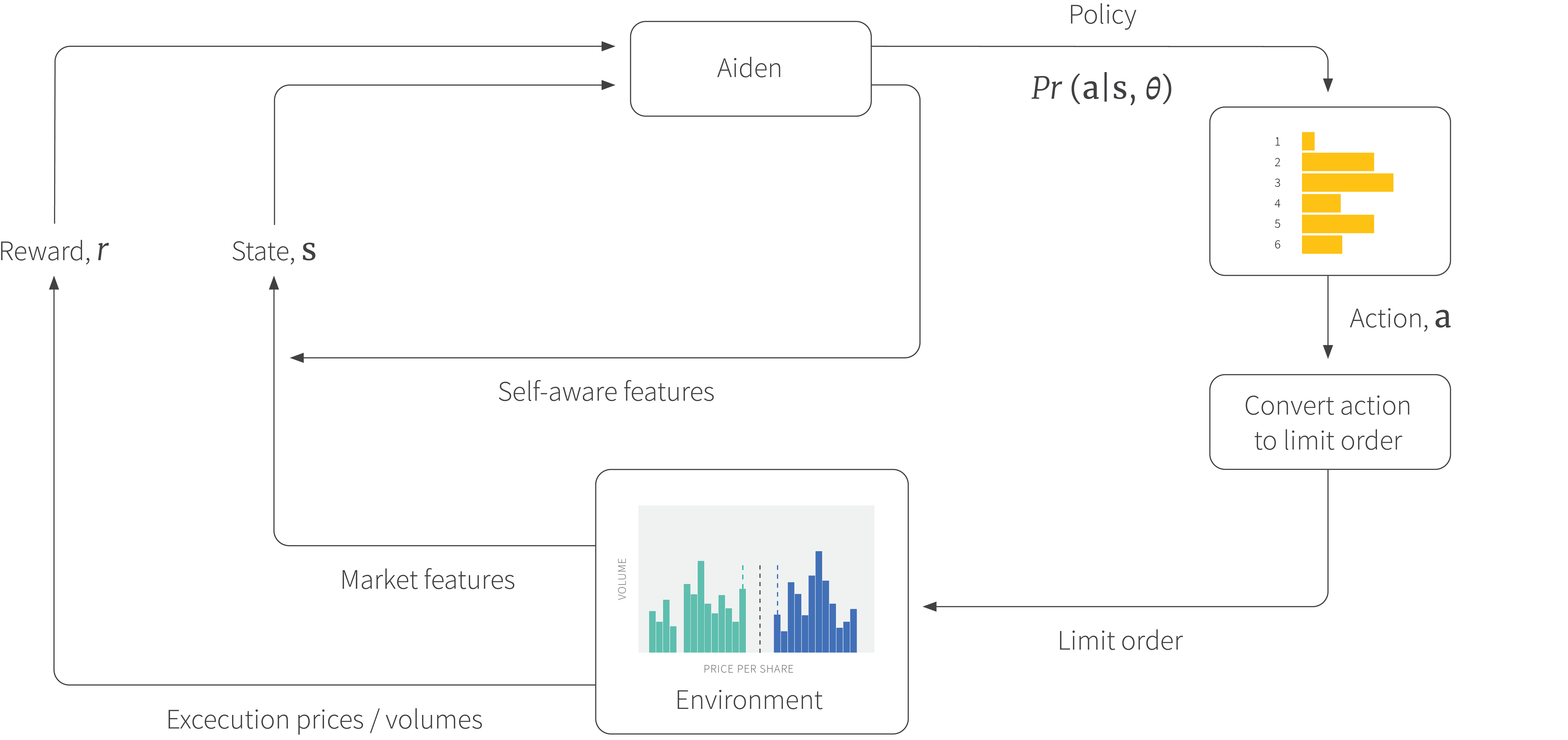
Figure 5. Aiden reinforcement learning overview. Aiden predicts the policy which is a distribution over several possible actions that relate to the aggressiveness of the order. One action is drawn randomly from this distribution and this is then converted to a limit order. This order is entered into the limit order book (environment). Placing the order affects the environment and produces a reward. The contents of the limit order book are summarized by a set of market features. The state consists of these market features plus a set of self-aware features that capture Aiden’s recent behaviour. Both the reward and the state are passed back to Aiden which predicts the next policy.
Proximal policy optimization
Aiden exploits another trick to make learning more stable in that is uses proximal policy optimization. This method changes the objective function to:
\begin{equation} J[\boldsymbol\theta] = \mathbb{E}\left[\frac{Pr(\mathbf{a}_{t}|\mathbf{s}_{t},\boldsymbol\theta)}{Pr(\mathbf{a}_{t}|\mathbf{s}_{t},\boldsymbol\theta_{old})}\Psi_{t} \right], \tag{2}\end{equation}
where the term $\boldsymbol\theta_{old}$ represents the parameters before the update and then clips this function to prevent very large changes in the policy (hence making it more stable). Defining:
\begin{equation} f[\boldsymbol\theta] = \frac{Pr(\mathbf{a}_{t}|\mathbf{s}_{t},\boldsymbol\theta)}{Pr(\mathbf{a}_{t}|\mathbf{s}_{t},\boldsymbol\theta_{old})}, \tag{3}\end{equation}
proximal policy optimization maximizes the following surrogate objective:
\begin{equation} J[\boldsymbol\theta] = \begin{cases}\mathbb{E}\left[\min\left[ f[\boldsymbol\theta] \Psi_{t}, 1+\epsilon\right]\Psi_{t}\right] &\quad \Psi_{t} > 0 \\ \mathbb{E}\left[\max\left[ f[\boldsymbol\theta] \Psi_{t}, 1-\epsilon\right]\Psi_{t}\right] &\quad \Psi_{t} \leq 0, \end{cases} \tag{4}\end{equation}
where $\epsilon$ is a pre-defined threshold.
Training
In this section we discuss a few of the challenges of training a production-level system for the order execution problem like Aiden.
Generality: The algorithm is required to work in many situations. Hence, the Aiden algorithm only uses input features that can be found in any market. Moreover, different stocks vary in price, liquidity, volatility and other quantities. To this end, the Aiden algorithm must normalize the input features so that the absolute magnitudes of price and volume observed in the market micro-structure data are factored out.
Simulation: Reinforcement learning algorithms are notorious for the amount of data that they must consume to learn a successful strategy. Obviously, it’s not practical to wait many years for the algorithm to train. Furthermore, we cannot put the algorithm into the real marketplace before it has learned which decisions to make to achieve good performance.
The solution to both of these problems is to build a training environment in which the market can be simulated based on observations of historical trading data. In this way, Aiden can train much faster than real-time and learn sensible policies without risking financial loss. This procedure can be sped up even more by training multiple RL agents who compete with one another in the same simulated market and learn from one another.
Conclusion
In this article we introduced the order execution problem and showed how it could be mapped to a reinforcement learning problem. We then described some features of Aiden, RBC’s electronic execution platform. The scope for reinforcement learning in finance is huge since there are often many rapid decisions that need to be made and these need to take into account the present condition of the market. Aiden is one of the first steps in RBC’s adoption of these technologies.