
This blog is the fifth in a series in which we consider machine learning from four different viewpoints. We either use gradient descent or a fully Bayesian approach and for each, we can choose to focus on either the model parameters or the output function (figure 1). In part I, part II, and part III, we considered gradient descent in both parameter and function space; this led to the development of the neural tangent kernel.
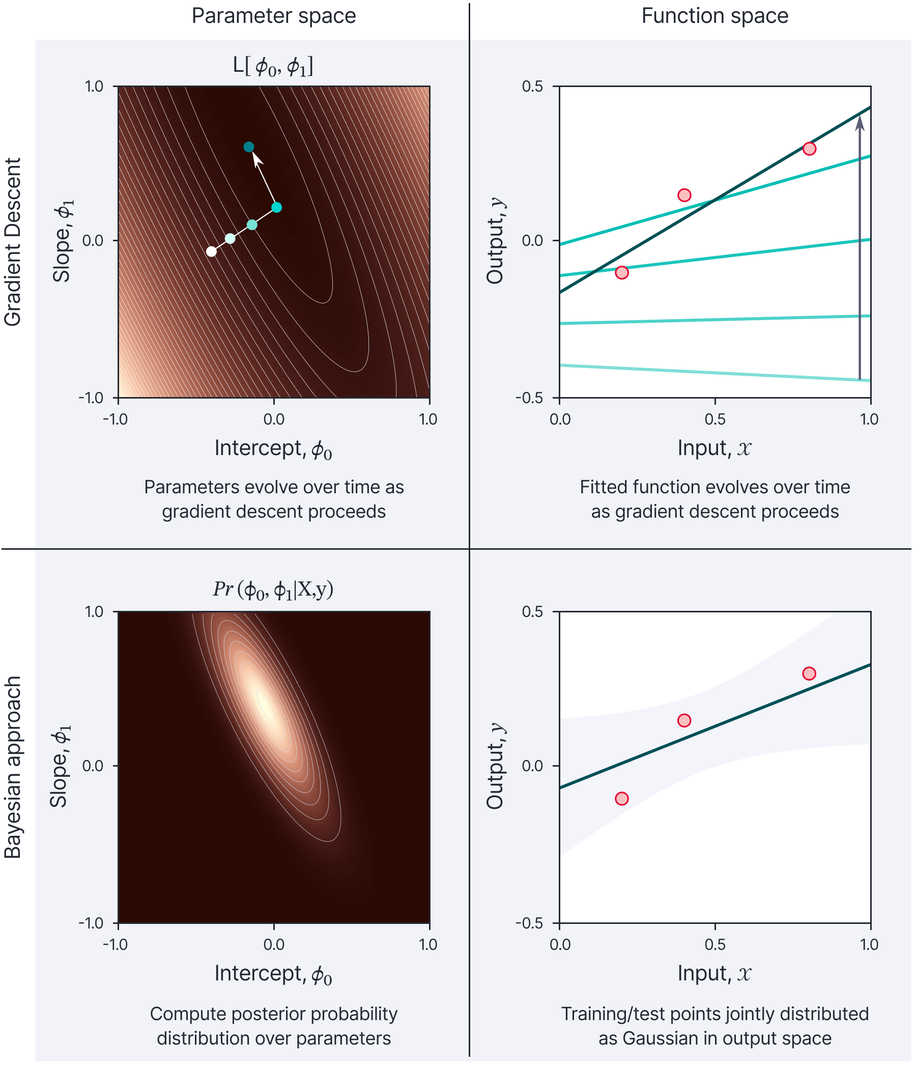
Figure 1. Four approaches to model fitting. We can either consider gradient descent (top row) or a Bayesian approach (bottom row). For either, we can consider either parameter space (left column) or the function space (right column). This blog will consider the Bayesian approach in function space (lower-right panel). Figure inspired by Sohl-Dickstein (2021).
In part IV of the series we considered the Bayesian approach to model fitting in a simple linear regression model from the perspective of parameter space. Here, we determine a probability distribution over possible parameter values rather than choosing a single “best” estimate. To make a prediction, we take a weighted average the predictions from all possible parameter estimates, where the weights are based on these probabilities. This scheme has the merits of (i) making more moderate predictions and (ii) providing estimates of uncertainty over these predictions.
In this (part V) of this series, we investigate the Bayesian approach from the perspective of function space. This is considerably simpler than the parameter space view and, for linear regression, results in the same predictions. However, as we shall see in the subsequent parts of this series, the implications of the two viewpoints are quite different for neural network models.
This blog is accompanied by a CoLab Python Notebook.
Function Space
In the function space view, we convert the prior $Pr(\boldsymbol\phi)$ over the model parameters $\boldsymbol\phi$ space into a prior $\operatorname{Pr}(\mathbf{f})$ over the function $\textbf{f}[\bullet]$ itself. This allows us to define a joint probability distribution between the function values for the training data and that for the test data. We then compute the conditional distribution of the function value for the test data given the training data.
Linear Model
These ideas are easiest to understand with the concrete example of the linear model:
\begin{align*}
y & =\mathrm{f}[\mathbf{x}, \boldsymbol{\phi}] \\
& =\mathbf{x}^{T} \boldsymbol{\phi}, \tag{1}
\end{align*}
where $\mathbf{x} \in \mathbb{R}^{D}$ is the input data, $y \in \mathbb{R}$ is the model output and $\boldsymbol{\phi} \in \mathbb{R}^{D}$ contains the parameters. As usual, we append the value one to the input data so that $\mathbf{x} \leftarrow$ $\left[\mathbf{x}^{T}, 1\right]^{T}$ to account for the y-offset.
As before, we’ll concatenate all of the $I$ training inputs $\mathbf{x}_{i} \in \mathbb{R}^{D}$ into a single matrix $\mathbf{X} \in \mathbb{R}^{D \times I}$, all of the function outputs $\mathrm{f}[\mathbf{x}, \boldsymbol{\phi}] \in \mathbb{R}$ into a single column vector $\mathbf{f} \in \mathbb{R}^{I}$ and all of the training outputs $y_{i} \in \mathbb{R}$ into a single column vector $\mathbf{y} \in$ $\mathbb{R}^{I}$. We can then write the model in two stages:
\begin{align*}
\mathbf{f} & =\mathbf{X}^{T} \boldsymbol{\phi} \\
\operatorname{Pr}(\mathbf{y} \mid \mathbf{f}) & =\operatorname{Norm}_{\mathbf{y}}\left[\mathbf{f}, \sigma_{n}^{2} \mathbf{I}\right], \tag{2}
\end{align*}
where as before $\sigma_{n}^{2}$ is the noise variance that accounts for the fact that the observed data are not exactly fitted by the model.
Prior distribution
We define a prior distribution over the parameters. As for the parameter-space perspective, we choose a spherical normal distribution with mean zero, and variance $\sigma_{p}^{2}$:
\begin{equation*}
\operatorname{Pr}(\boldsymbol\phi)=\operatorname{Norm}_{\boldsymbol{\phi}}\left[\mathbf{0}, \sigma_{p}^{2} \mathbf{I}\right]. \tag{3}
\end{equation*}
This is illustrated in figure 2a
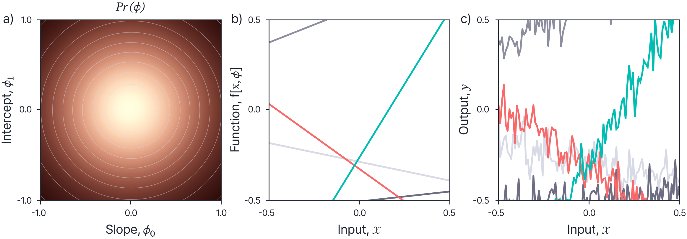
Figure 2. Prior over parameters for 1D regression model. a) The prior for the parameters $\phi_{0}, \phi_{1}$ of a 1D regression model $y=\phi_{0} x+\phi_{1}$ is typically defined as a standard normal distribution with mean zero and a broad covariance $\sigma_{p}^{2} \mathbf{I}$. b) Five samples from the prior; each represents a single choice of parameters $\phi$ and hence defines an input/output mapping $\mathrm{f}[\mathbf{x}, \boldsymbol{\phi}]$. These examples, can alternatively be drawn directly from a prior $\operatorname{Pr}(\mathbf{f})$ over the functions space. c) The model outputs y typically have added noise with variance $\sigma_{w}^{2}$.
Gaussian processes
Now we note that the function values $\mathbf{f}=\mathbf{X}^{T} \boldsymbol{\phi}$ are an affine transform of the parameters, and we use the relation (see proof at end of blog) that if $\operatorname{Pr}(\mathbf{z})=$$\operatorname{Norm}_{\mathbf{z}}[\boldsymbol{\mu}, \boldsymbol{\Sigma}]$, then the affine transform $\mathbf{a}+\mathbf{B z}$ is distributed as:
\begin{equation*}
\operatorname{Pr}(\mathbf{a}+\mathbf{B z})=\operatorname{Norm}\left[\mathbf{a}+\mathbf{B} \boldsymbol{\mu}, \mathbf{B} \boldsymbol{\Sigma} \mathbf{B}^{T}\right]. \tag{4}
\end{equation*}
Applying this relation, we can get a prior distribution over the function values $\mathbf{f}$:
\begin{equation*}
\operatorname{Pr}(\mathbf{f} \mid \mathbf{X})=\operatorname{Norm}_{\mathbf{f}}\left[\mathbf{0}, \sigma_{p}^{2} \mathbf{X}^{T} \mathbf{X}\right]. \tag{5}
\end{equation*}
This is technically a Gaussian process, and can equivalently be written as:
\begin{equation*}
\mathbf{f}[\mathbf{X}] \sim \mathcal{G P}\left[\mathbf{0}, \sigma_{p}^{2} \mathbf{X}^{T} \mathbf{X}\right]. \tag{6}
\end{equation*}
The term Gaussian process just refers to a collection of random variables, any finite number of which have a joint Gaussian distribution (see Rasmussen and Williams, 2006). In this case, we can define any input values $\mathbf{X}$ and equation 6 defines a Gaussian distribution between them. For example, we can define a set of equally spaced 1D points and draw samples $\mathbf{f}$ from this prior. Each sample looks like a straight line (figure 2b).
Since the output $\mathbf{y}$ is just a noisy version of the function values, we can similarly write a prior distribution over the output values:
\begin{equation*}
\operatorname{Pr}(\mathbf{y} \mid \mathbf{X})=\operatorname{Norm}_{\mathbf{f}}\left[\mathbf{0}, \sigma_{p}^{2} \mathbf{X}^{T} \mathbf{X}+\sigma_{n}^{2} \mathbf{I}\right]. \tag{7}
\end{equation*}
Figure 2c illustrates samples drawn from this distribution for a set of equally spaced inputs.
Inference
Consider a test set of points $\mathbf{X}^{*}$ which map to function values $\mathbf{f}^{*}$. We can write the joint distribution of the training values $\mathbf{y}$ and the new function value $\mathbf{f}^{*}$:
\[
\operatorname{Pr}\binom{\mathbf{y}}{\mathbf{f}^{*}}=\operatorname{Norm}_{\left[\mathbf{y},\mathbf{f}^{*} \right]^{T}}\left[\left[\begin{array}{l}
0 \tag{8}\\
0
\end{array}\right],\left[\begin{array}{cc}
\sigma_{p}^{2} \mathbf{X}^{* T} \mathbf{X}^{*} & \sigma_{p}^{2} \mathbf{X}^{* T} \mathbf{X} \\
\sigma_{p}^{2} \mathbf{X}^{T} \mathbf{X}^{*} & \sigma_{p}^{2} \mathbf{X}^{T} \mathbf{X}+\sigma_{n}^{2} \mathbf{I}
\end{array}\right]\right].
\]
Now we use the following well-known relation for conditional distributions in Gaussian variables (proof at end of blog): if two sets of variables $\mathbf{z}_{1}$ and $\mathbf{z}_{2}$ are jointly distributed as a multivariate normal:
\[
\operatorname{Pr}\left(\left[\begin{array}{l}
\mathbf{z}_{1} \tag{9}\\
\mathbf{z}_{2}
\end{array}\right]\right)=\operatorname{Norm}_{\mathbf{z}}\left[\left[\begin{array}{l}
\boldsymbol{\mu}_{1} \\
\boldsymbol{\mu}_{2}
\end{array}\right],\left[\begin{array}{ll}
\boldsymbol{\Sigma}_{11} & \boldsymbol{\Sigma}_{12} \\
\boldsymbol{\Sigma}_{21} & \boldsymbol{\Sigma}_{22}
\end{array}\right]\right],
\]
then the conditional distribution of $\mathbf{z}_{2}$ given observed values $\mathbf{z}_{1}$ is:
\begin{equation*}
\operatorname{Pr}\left(\mathbf{z}_{1} \mid \mathbf{z}_{2}\right)=\operatorname{Norm}_{\mathbf{z}_{1}}\left[\boldsymbol{\mu}_{\mathbf{1}}+\boldsymbol{\Sigma}_{12} \boldsymbol{\Sigma}_{22}^{-1}\left(\mathbf{z}_{2}-\boldsymbol{\mu}_{2}\right), \boldsymbol{\Sigma}_{11}-\boldsymbol{\Sigma}_{12} \boldsymbol{\Sigma}_{22}^{-1} \boldsymbol{\Sigma}_{12}^{T}\right]. \tag{10}
\end{equation*}
Applying this relation to equation 8, we get:
\begin{align*}
\operatorname{Pr}\left(\mathbf{f}^{*} \mid \mathbf{X}^{*}, \mathbf{X}, \mathbf{y}\right)&= \operatorname{Norm}_{\mathbf{f}^{*}}\left[\sigma_{p}^{2} \mathbf{X}^{* T} \mathbf{X}\left(\sigma_{p}^{2} \mathbf{X}^{T} \mathbf{X}+\sigma_{n}^{2} \mathbf{I}\right)^{-1} \mathbf{y}\right., \tag{11}\\
&\hspace{3cm}\left.\sigma_{p}^{2} \mathbf{X}^{* T} \mathbf{X}^{*}-\sigma_{p}^{2} \mathbf{X}^{* T} \mathbf{X}\left(\sigma_{p}^{2} \mathbf{X}^{T} \mathbf{X}+\sigma_{n}^{2} \mathbf{I}\right)^{-1} \sigma_{p}^{2} \mathbf{X}^{T} \mathbf{X}^{*}\right] \\
&= \operatorname{Norm}_{\mathbf{f}^{*}}\Biggl[\mathbf{X}^{* T} \mathbf{X}\left(\mathbf{X}^{T} \mathbf{X}+\frac{\sigma_{n}^{2}}{\sigma_{p}^{2}} \mathbf{I}\right)^{-1} \mathbf{y}, \\
&\hspace{3cm}\sigma_{p}^{2} \mathbf{X}^{* T} \mathbf{X}^{*}-\sigma_{p}^{2} \mathbf{X}^{* T} \mathbf{X}\left(\mathbf{X}^{T} \mathbf{X}+\frac{\sigma_{n}^{2}}{\sigma_{p}^{2}} \mathbf{I}\right)^{-1} \mathbf{X}^{T} \mathbf{X}^{*}\Biggr]
\end{align*}
where we have moved the terms $\sigma_{p}^{2}$ into the inverse in the second line. If we draw samples from this distribution for equally spaced test points in $\mathbf{X}^{*}$, each sample looks like a line that is broadly compatible with the training data $\mathbf{X}$ (figure 3a).
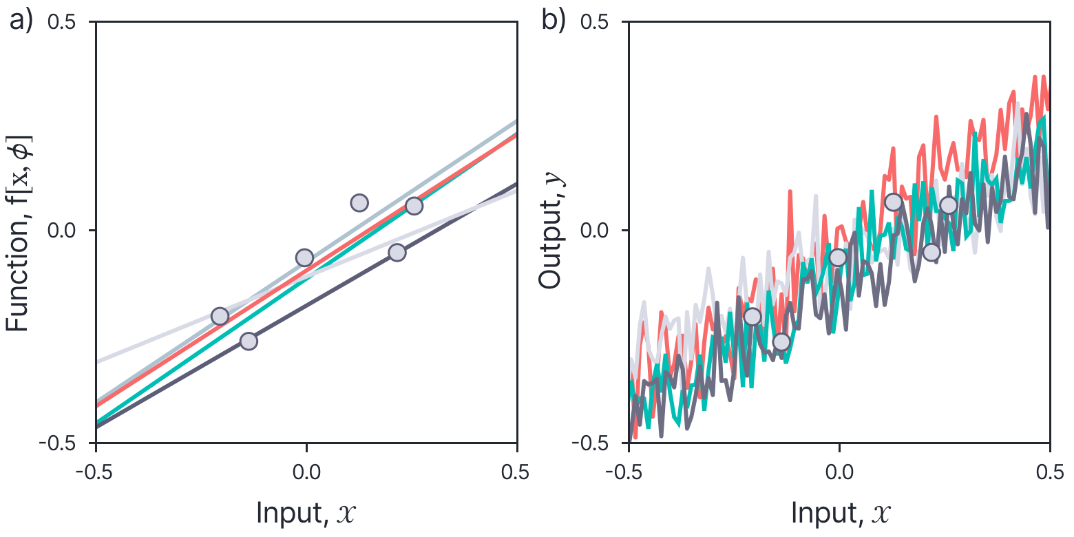
Figure 3. Samples from posterior distribution over functions $\operatorname{Pr}\left(\mathbf{f}^{*} \mid \mathbf{X}^{*}, \mathbf{X}, \mathbf{y}\right)$ conditioned on six observed data points $\left\{\mathbf{x}_{i}, y_{i}\right\}$ (stored in $\mathbf{X}$ and $\mathbf{y}$. Each looks like a line that is broadly compatible with the data. b) Samples from output function; these are the same, but with added noise $\sigma_{n}^{2}$; we expect the observed data points to be samples from this distribution.
Finally, we note that the original data points are drawn from distribution over the noisy output $\mathbf{y}^{*}$, which has the same distribution plus an the extra noise term on the covariance.
\begin{align*}
& \operatorname{Pr}\left(\mathbf{y}^{*} \mid \mathbf{X}^{*}, \mathbf{X}, \mathbf{y}\right)=\operatorname{Norm}_{\mathbf{y}^{*}} {\Biggl[\mathbf{X}^{* T} \mathbf{X}\left(\mathbf{X}^{T} \mathbf{X}+\frac{\sigma_{n}^{2}}{\sigma_{p}^{2}} \mathbf{I}\right)^{-1} \mathbf{y}} \\
&\hspace{3cm}\sigma_{p}^{2} \mathbf{X}^{* T} \mathbf{X}^{*}-\sigma_{p}^{2} \mathbf{X}^{* T} \mathbf{X}\left(\mathbf{X}^{T} \mathbf{X}+\frac{\sigma_{n}^{2}}{\sigma_{p}^{2}} \mathbf{I}\right)^{-1} \mathbf{X}^{T} \mathbf{X}^{*}+\sigma_{n}^{2} \mathbf{I}\Biggl]. \tag{12}
\end{align*}
Samples from this distribution look like noisy lines that are broadly compatible with the data points (figure 3b).
Figure 4 visualizes the solution in a different way. Here, we have plotted the mean of the posterior (the MAP solution) and the marginal uncertainty at each of a set of equally spaced positions (represented by a $\pm 2$ standard deviation region). In this way, we can visualize the function and its uncertainty, or the equivalent result in output space.
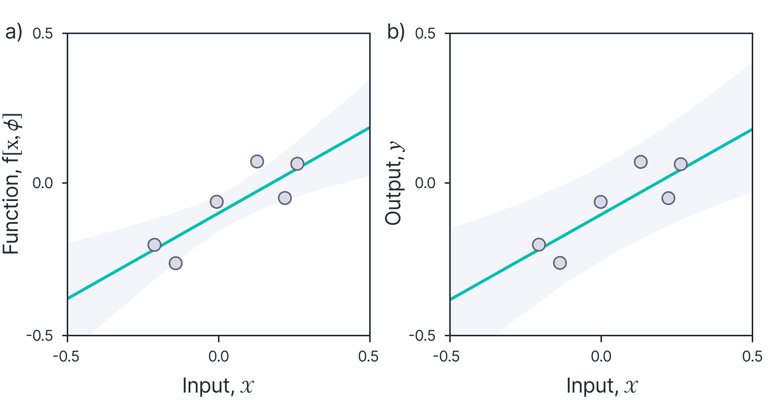
Figure 4. Posterior distribution with marginal uncertainty. a) The function predictions can also be visualized as the mean of the posterior distribution (the MAP solution, cyan line) and the marginal uncertainty at each input point (represented by $\pm 2$ standard deviation region). The uncertainty increases as we extrapolate further from the data. b) The noisy output predictions can be visualized in the same way but have additional noise $\sigma_{n}^{2}$ at each point. The observed data points will usually fall within the $\pm 2$ standard deviation region.
Parameter space vs. function space
Recall from part IV of this series of blogs that the predictive distribution for the parameter space (Bayesian) view of the linear model was:
\begin{align*}
\operatorname{Pr}\left(y^{*} \mid \mathbf{x}^{*}, \mathbf{X}, \mathbf{y}\right)=\operatorname{Norm}_{y^{*}}\Biggl[ & \mathbf{x}^{* T} \mathbf{X}\left(\mathbf{X}^{T} \mathbf{X}+\frac{\sigma_{n}^{2}}{\sigma_{p}^{2}} \mathbf{I}\right)^{-1} \mathbf{y} \tag{13}\\
& \sigma_{p}^{2} \mathbf{x}^{* T} \mathbf{x}^{*}-\sigma_{p}^{2} \mathbf{x}^{* T} \mathbf{X}\left(\mathbf{X}^{T} \mathbf{X}+\frac{\sigma^{2}}{\sigma_{p}^{2}} \mathbf{I}\right)^{-1} \mathbf{X}^{T} \mathbf{x}^{*}+\sigma_{n}^{2}\Biggr].
\end{align*}
It’s clear that for this model, the parameter space view and the function space view lead to the same result (although we developed the function space approach to make multiple predictions simultaneously). However, this is NOT true in general. In future articles in this series, we will see that these two perspectives have quite different implications for neural networks.
Non-linear regression
For both the parameter space and function space views, we only yield neat closed-form solution for the predictions because the model is linear; although the same principles apply for non-linear models, there is not generally a closed-form solution. What then, should we do when faced with a training dataset for which a linear model is clearly inadequate? One tractable approach is to transform the initial data by a fixed non-linear transformation $\mathbf{z}=\mathbf{g}[\mathbf{x}]$ and then apply a linear model $\mathrm{f}[\mathbf{z}, \boldsymbol{\phi}]$ to the transformed data.
Example: polynomial regression
A simple example of this type of model is polynomial regression for 1D data $x$ in which we might use the non-linear transformation (figure 2a):
\[
\mathbf{z}=\left[\begin{array}{c}
1 \tag{2}\\
x \\
x^{2} \\
x^{3} \\
x^{4}
\end{array}\right].
\]
If we draw samples from the prior from this model, each looks like a polynomial of order five (figure 5).

Figure 5. Polynomial model. a) The input data $x$ is transformed by a fixed non-linearity to create a new input vector $\mathbf{z}$ which is then passed into the linear model. Here the 1D data $x$ is transformed to a 5D vector consisting of the first four polynomial basis functions and the constant function (not shown). b) If we define a prior over the model parameters $\phi$, then we can draw samples from the induced prior over functions. Each looks like a random fourth-order polynomial.
When we condition the output function on a training dataset, we samples from the posterior look like order-5 polynomial curves that broadly agree with the data (figure 6a), or we can alternatively visualize the MAP solution and the associated marginal uncertainty (figure 6b).
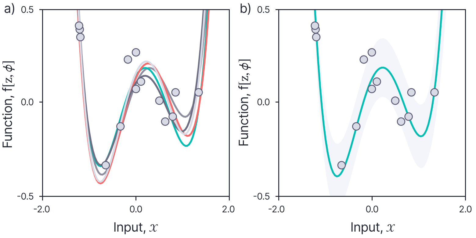
Figure 6. Posterior distribution for polynomial model. a) If we condition the function on a set of observed data points, we can compute a posterior distribution over the function values. Each curve represents a sample from this distribution. b) As before, we can visualize this distribution using the MAP sample (blue line) and the marginal variance (gray region).
In this way, we can make closed-form predictions based on a polynomial model and yield estimates of uncertainty, without ever explicitly ‘fitting’ the model and committing to a single set of parameters.
Example: ReLU model
A second example is a transformation based on a collection of offset ReLU functions:
\[
\mathbf{z}=\left[\begin{array}{c}
1 \tag{15}\\
\operatorname{ReLU}\left[\beta_{1}+\omega_{1} x\right] \\
\operatorname{ReLU}\left[\beta_{2}+\omega_{2} x\right] \\
\operatorname{ReLU}\left[\beta_{3}+\omega_{3} x\right] \\
\operatorname{ReLU}\left[\beta_{4}+\omega_{4} x\right] \\
\operatorname{ReLU}\left[\beta_{5}+\omega_{5} x\right]
\end{array}\right].
\]
Note that this is not exactly the same as a neural network because in this case the biases $\beta_{0}$ and slopes $\omega_{0}$ are chosen in advance and fixed; they are not optimized (or marginalized over) as part of the training process.
The prior and posterior functions are visualized in figure 7 and 8, respectively. In each case the output function is a piecewise linear, with the position of the joints determined by the joints in the component ReLU functions (which are themselves determined by the predefined $\beta_{\bullet}$ and $\omega_{\bullet}$ parameters.
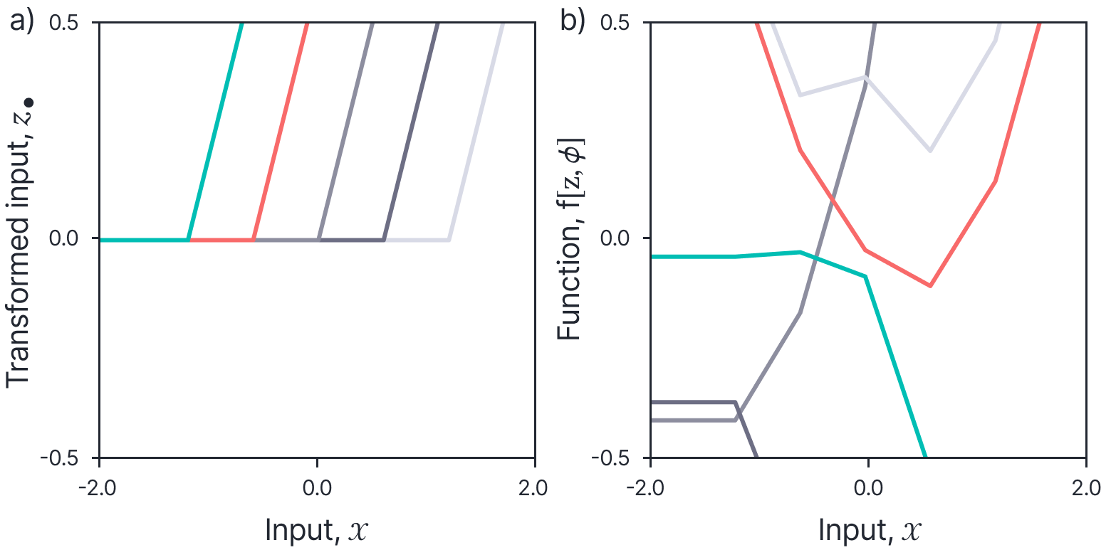
Figure 7. ReLU model. a) The input data $x$ is transformed by a fixed non-linearity to create a new input vector $\mathbf{z}$ which is then passed into the linear model. Here the 1D data $x$ is transformed to a 6D vector consisting of the five horizontally offset ReLU functions and the constant function (not shown). b) If we define a prior over the model parameters $\phi$, then we can draw samples from the induced prior over functions. Each looks like a piecewise linear function where the position of the joints is determined by the component ReLU functions.
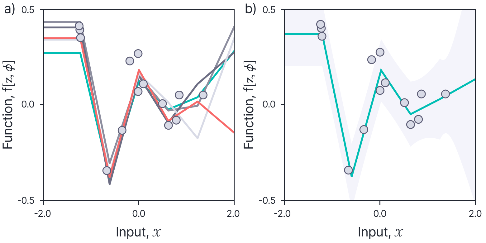
Figure 8. Posterior distribution for ReLU model. a) If we condition the function on a set of observed data points, we can compute a posterior distribution over the function values. Each curve represents a sample from this distribution. b) As before, we can visualize this distribution using the MAP sample (blue line) and the marginal variance (gray region).
Disadvantages of non-linear regression
Although, the approach of transforming the input data using a fixed non-linearity is simple and effective, these methods do not necessarily scale well to high dimensions. For example, if we have 1000 dimensional input, then the set of third degree polynomials contains $\left(D_{z}=1+1000+1000^{2}+1000^{3}\right)$ terms. However, the complexity of the fitted function should ultimately depend on the amount of training data. If this is significantly less than the number of transformed dimensions, we should be able to make efficiency gains.
Kernels and the kernel trick
To make progress, we note that the final equation for the predictive distribution:
\begin{align*}
\operatorname{Pr}\left(\mathbf{y}^{*} \mid \mathbf{Z}^{*}, \mathbf{Z}, \mathbf{y}\right)=\operatorname{Norm}_{\mathbf{y}^{*}} & {\Biggl[\mathbf{Z}^{* T} \mathbf{Z}\left(\mathbf{Z}^{T} \mathbf{Z}+\frac{\sigma_{n}^{2}}{\sigma_{p}^{2}} \mathbf{I}\right)^{-1} \mathbf{y}}, \\
& \sigma_{p}^{2} \mathbf{Z}^{* T} \mathbf{Z}^{*}-\sigma_{p}^{2} \mathbf{Z}^{* T} \mathbf{Z}\left(\mathbf{Z}^{T} \mathbf{Z}+\frac{\sigma_{n}^{2}}{\sigma_{p}^{2}} \mathbf{I}\right)^{-1} \mathbf{Z}^{T} \mathbf{Z}^{*}+\sigma_{n}^{2} \mathbf{I}\Biggr] \tag{16}
\end{align*}
depends only on matrix products of the form $\mathbf{Z}^{T} \mathbf{Z}$ where $\mathbf{Z} \in \mathbb{R}^{D_{z} \times I}$ contains the transformed data vectors in its columns.
When the dimension $D_{z}$ of the transformed vectors $\mathbf{z}=\mathbf{g}[\mathbf{x}]$ is high, computing the non-linear transformations and computing the dot products that make the matrix product can be time-consuming. A viable alternative is kernel substitution in which we directly define a single kernel function $\mathrm{k}\left[\mathbf{x}_{i}, \mathbf{x}_{j}\right]$ as a replacement for the operations $\mathbf{g}\left[\mathbf{x}_{i}\right]^{T} \mathbf{g}\left[\mathbf{x}_{j}\right]$. For many transformations $\mathbf{g}[\bullet]$ it is more efficient to evaluate the kernel function directly than to transform the variables separately and then compute the dot product.
Taking this idea one step further, it is possible to choose a kernel function $\mathrm{k}\left[\mathbf{x}_{i}, \mathbf{x}_{j}\right]$ without knowledge of what transformation $\mathbf{g}[\bullet]$ it corresponds to. Clearly, the function must be carefully chosen so that it does in fact correspond to computing some function $\mathbf{z}=\mathbf{g}[\mathbf{x}]$ of each data vector and taking the inner product of the results: for example, since $\mathbf{z}_{i}^{T} \mathbf{z}_{j}=\mathbf{z}_{j}^{T} \mathbf{z}_{i}$ it must treat its arguments symmetrically so that $\mathrm{k}\left[\mathbf{x}_{i}, \mathbf{x}_{j}\right]=\mathrm{k}\left[\mathbf{x}_{j}, \mathbf{x}_{i}\right]$.
When we use kernel functions, we no longer explicitly compute the transformed vector $\mathbf{z}$. One advantage of this is we can define kernel functions that correspond to projecting the data into very high dimensional or even infinite spaces.
We now return to the question of which constraints must be put on the kernel function to ensure that there exists an underlying function $\mathbf{f}\left[\mathbf{x}_{i}\right]=\mathbf{z}_{i}$ so that $\mathrm{k}\left[\mathbf{x}_{i}, \mathbf{x}_{j}\right]=\mathbf{z}_{i}^{T} \mathbf{z}_{j}$. Mercer’s theorem states that this is true when the kernel’s arguments are in a measurable space, and the kernel is positive semi-definite so that:
\begin{equation*}
\sum_{i j} \mathrm{k}\left[\mathbf{x}_{i}, \mathbf{x}_{j}\right] a_{i} a_{j} \geq 0, \tag{17}
\end{equation*}
for any finite subset $\left\{\mathbf{x}_{n}\right\}_{n=1}^{N}$ of vectors in the space and any real numbers $\left\{a_{n}\right\}_{n=1}^{N}$. Examples of valid kernels include:
- Linear:
\begin{equation*}
\mathrm{k}\left[\mathbf{x}_{i}, \mathbf{x}_{j}\right]=\mathbf{x}_{i}^{T} \mathbf{x} \tag{18}
\end{equation*} - Degree $p$ polynomial:
\begin{equation*}
\mathrm{k}\left[\mathbf{x}_{i}, \mathbf{x}_{j}\right]=\left(\mathbf{x}_{i}^{T} \mathbf{x}_{j}+1\right)^{p} \tag{19}
\end{equation*} - Radial basis function (RBF) or Gaussian:
\begin{equation*}
\mathrm{k}\left[\mathbf{x}_{i}, \mathbf{x}_{j}\right]=\exp \left[-0.5\left(\frac{\left(\mathbf{x}_{i}-\mathbf{x}_{j}\right)^{T}\left(\mathbf{x}_{i}-\mathbf{x}_{j}\right)}{\lambda^{2}}\right)\right] \tag{20}
\end{equation*}
The last of these is particularly interesting. It can be shown that this kernel function corresponds to computing infinite length vectors $\mathbf{z}$ and taking their dot product. The entries of $\mathbf{z}$ correspond to evaluating a radial basis function at every possible point in the space of $\mathbf{x}$.
It is also possible to create new kernels by combining two or more existing kernels. For example, sums and products of valid kernels are guaranteed to be positive semi-definite and so are also valid kernels.
Using kernel notation, we can now write the predictive equation as:
\begin{align*}
& \operatorname{Pr}\left(\mathbf{y}^{*} \mid \mathbf{X}^{*}, \mathbf{X}, \mathbf{y}\right)=\operatorname{Norm}_{\mathbf{y}^{*}}\Biggl[\mathbf{K}[\mathbf{X}, \mathbf{X}]\left(\mathbf{K}[\mathbf{X}, \mathbf{X}]+\frac{\sigma_{n}^{2}}{\sigma_{p}^{2}} \mathbf{I}\right)^{-1} \mathbf{y}, \\
& \hspace{2cm}\quad \sigma_{p}^{2} \mathbf{K}\left[\mathbf{X}^{*}, \mathbf{X}^{*}\right]-\sigma_{p}^{2} \mathbf{K}\left[\mathbf{X}^{*}, \mathbf{X}\right]\left(\mathbf{K}[\mathbf{X}, \mathbf{X}]+\frac{\sigma_{n}^{2}}{\sigma_{p}^{2}} \mathbf{I}\right)^{-1} \mathbf{K}\left[\mathbf{X}, \mathbf{X}^{*}\right]+\sigma_{n}^{2} \mathbf{I}\Biggr], \tag{21}
\end{align*}
where the $(i, j)^{\text {th }}$ element of $\mathbf{K}\left[\mathbf{X}^{*}, \mathbf{X}\right]$ would comprise the element $\mathrm{k}\left[\mathbf{x}_{i}^{*}, \mathbf{x}_{j}\right]$ and so on. Figure 2.9 shows the prior and posterior distribution for kernel regression using the RBF kernel; it results in a set of smooth functions that pass close to the data points.
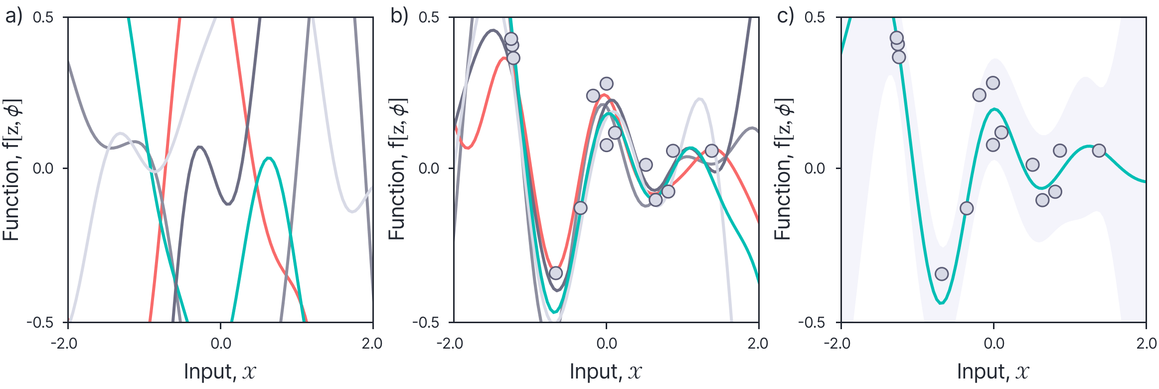
Figure 9. Kernel regression with RBF kernel. a) Samples from the prior distribution over functions look like smooth curves (the speed of change is determined by the kernel parameter $\lambda$). b) Samples from the posterior look like smooth functions that pass through the training data. c) This posterior can also be visualized as the MAP function and the marginal uncertainty.
Conclusion
In this blog we described a method to define a prior over the space of output functions. We can use this prior find a joint distribution over the training and test data points; we then find the conditional distribution over the test points, given the training points. For linear models, this gives the same results as the parameter-space perspective on Bayesian modelling. We saw how this approach can be extended to model more complex data by applying a non-linear transformation to the input data before applying the linear model.
The next part of this series of blogs applies the Bayesian approach to deep neural networks. We will see that the implications of parameter-space and function-space perspectives are quite different here.
Affine transformations of normal distributions
The multivariate normal distribution is defined as:
$$
\operatorname{Pr}(\mathbf{x})=\frac{1}{(2 \pi)^{D}|\boldsymbol{\Sigma}|^{1 / 2}} \exp \left[-0.5(\mathbf{x}-\boldsymbol{\mu}) \boldsymbol{\Sigma}^{-1}(\mathbf{x}-\boldsymbol{\mu})\right].
$$
To transform the distribution as $\mathbf{y}=\mathbf{A} \mathbf{x}+\mathbf{b}$, we substitute in $\mathbf{x}=\mathbf{A}^{-1}(\mathbf{y}-\mathbf{b})$ and divide by the determinant of the Jacobian of the transformation, which for this case is just $|\mathbf{A}|$ giving:
$$
\operatorname{Pr}(\mathbf{x})=\frac{1}{(2 \pi)^{D}|\boldsymbol{\Sigma}|^{1 / 2}|\mathbf{A}|} \exp \left[-0.5\left(\mathbf{A}^{-1}(\mathbf{y}-\mathbf{b})-\boldsymbol{\mu}\right) \boldsymbol{\Sigma}^{-1}\left(\mathbf{A}^{-1}(\mathbf{y}-\mathbf{b})-\boldsymbol{\mu}\right)\right].
$$
We’ll first work with the constant $\kappa$ from outside the exponential to show that it is the constant for a distribution with variance $\mathbf{A} \boldsymbol{\Sigma} \mathbf{A}^{T}$. We have:
\begin{aligned}
\kappa & =\frac{1}{(2 \pi)^{D}|\mathbf{\Sigma}|^{1 / 2}|\mathbf{A}|} \\
& =\frac{1}{(2 \pi)^{D}|\mathbf{\Sigma}|^{1 / 2}|\mathbf{A}|^{1 / 2}|\mathbf{A}|^{1 / 2}} \\
& =\frac{1}{(2 \pi)^{D}|\mathbf{\Sigma}|^{1 / 2}|\mathbf{A}|^{1 / 2}\left|\mathbf{A}^{T}\right|^{1 / 2}} \\
& =\frac{1}{(2 \pi)^{D}|\mathbf{A}|^{1 / 2}|\mathbf{\Sigma}|^{1 / 2}\left|\mathbf{A}^{T}\right|^{1 / 2}} \\
& =\frac{1}{(2 \pi)^{D}\left|\mathbf{A} \mathbf{\Sigma} \mathbf{A}^{T}\right|^{1 / 2}},
\end{aligned}
which is exactly the required constant.
Now we’ll work with the quadratic in the exponential term to show that it corresponds to a normal distribution in $\mathbf{y}$ with variance $\mathbf{A} \boldsymbol{\Sigma} \mathbf{A}^{T}$ and mean $\mathbf{A} \boldsymbol{\mu}+\mathbf{b}$.
\begin{aligned}
\left(\mathbf{A}^{-1}(\mathbf{y}-\mathbf{b})-\boldsymbol{\mu}\right) \boldsymbol{\Sigma}^{-1}\left(\mathbf{A}^{-1}(\mathbf{y}-\mathbf{b})-\boldsymbol{\mu}\right) &\\
&\hspace{-4cm}=\mathbf{y}^{T} \mathbf{A}^{-T} \boldsymbol{\Sigma}^{-1} \mathbf{A}^{-1} \mathbf{y}-2\left(\mathbf{b}^{T} \mathbf{A}^{-T}+\boldsymbol{\mu}^{T}\right) \boldsymbol{\Sigma}^{-1} \mathbf{A}^{-1} \mathbf{y} \\
&+\left(\mathbf{A}^{-1} \mathbf{b}+\boldsymbol{\mu}\right)^{T} \boldsymbol{\Sigma}^{-1}\left(\mathbf{A}^{-1} \mathbf{b}+\boldsymbol{\mu}\right) \\
&\hspace{-4cm}=\mathbf{y}^{T} \mathbf{A}^{-T} \boldsymbol{\Sigma}^{-1} \mathbf{A}^{-1} \mathbf{y}-2\left(\mathbf{b}^{T}+\boldsymbol{\mu}^{T} \mathbf{A}^{T}\right) \mathbf{A}^{-T} \boldsymbol{\Sigma}^{-1} \mathbf{A}^{-1} \mathbf{y} \\
&+\left(\mathbf{A}^{-1} \mathbf{b}+\mathbf{A} \boldsymbol{\mu}\right)^{T} \mathbf{A}^{-T} \boldsymbol{\Sigma}^{-1} \mathbf{A}^{-1}(\mathbf{b}+\mathbf{A} \boldsymbol{\mu}) \\
&\hspace{-4cm}=(\mathbf{y}-(\mathbf{A} \boldsymbol{\mu}+\mathbf{b}))^{T}\left(\mathbf{A} \boldsymbol{\Sigma} \mathbf{A}^{T}\right)^{-1}(\mathbf{y}-(\mathbf{A} \boldsymbol{\mu}+\mathbf{b})).
\end{aligned}
This is clearly the quadratic term from a normal distribution in $\mathbf{y}$ with variance $\mathbf{A} \boldsymbol{\Sigma} \mathbf{A}^{T}$ and mean $\mathbf{A} \boldsymbol{\mu}+\mathbf{b}$ as required.
Conditional distribution of a Gaussian
Consider a joint Gaussian distribution with variables $\mathbf{z}=\left[\mathbf{z}_{1}, \mathbf{z}_{2}\right]$:
$$\operatorname{Pr}(\mathbf{z})=\operatorname{Pr}\left(\left[\begin{array}{l}
\mathbf{z}_{1} \\
\mathbf{z}_{2}
\end{array}\right]\right)=\operatorname{Norm}_{\mathbf{x}}\left[\left[\begin{array}{l}
\boldsymbol{\mu}_{1} \\
\boldsymbol{\mu}_{2}
\end{array}\right],\left[\begin{array}{ll}
\boldsymbol{\Sigma}_{11} & \boldsymbol{\Sigma}_{12} \\
\boldsymbol{\Sigma}_{21} & \boldsymbol{\Sigma}_{22}
\end{array}\right]\right].$$
The conditional distribution of the varaibles $\mathbf{z}_{1}$ given observed variables $\mathbf{z}_{2}$ is:
\begin{equation*}
\operatorname{Pr}\left(\mathbf{z}_{1} \mid \mathbf{z}_{2}\right)=\operatorname{Norm}_{\mathbf{z}_{1}}\left[\boldsymbol{\mu}_{\mathbf{1}}+\boldsymbol{\Sigma}_{12} \boldsymbol{\Sigma}_{22}^{-1}\left(\mathbf{z}_{2}-\boldsymbol{\mu}_{2}\right), \boldsymbol{\Sigma}_{11}-\boldsymbol{\Sigma}_{12} \boldsymbol{\Sigma}_{22}^{-1} \boldsymbol{\Sigma}_{12}^{T}\right]
\end{equation*}
Proof: We can write out the joint distribution as:
\begin{aligned}
\operatorname{Pr}\left(\left[\begin{array}{l}
\mathbf{z}_{1} \\
\mathbf{z}_{2}
\end{array}\right]\right) & =\kappa_{1} \exp \left[-0.5\left(\left[\begin{array}{l}
\mathbf{z}_{1} \\
\mathbf{z}_{2}
\end{array}\right]-\left[\begin{array}{l}
\boldsymbol{\mu}_{1} \\
\boldsymbol{\mu}_{2}
\end{array}\right]\right)^{T}\left[\begin{array}{ll}
\boldsymbol{\Sigma}_{11} & \boldsymbol{\Sigma}_{12} \\
\boldsymbol{\Sigma}_{12}^{T} & \mathbf{\Sigma}_{22}
\end{array}\right]^{-1}\left(\left[\begin{array}{l}
\mathbf{z}_{1} \\
\mathbf{z}_{2}
\end{array}\right]-\left[\begin{array}{l}
\boldsymbol{\mu}_{1} \\
\boldsymbol{\mu}_{2}
\end{array}\right]\right)\right] \\
& =\kappa_{1} \exp \left[-0.5\left(\left[\begin{array}{l}
\mathbf{z}_{1} \\
\mathbf{z}_{2}
\end{array}\right]-\left[\begin{array}{l}
\boldsymbol{\mu}_{1} \\
\boldsymbol{\mu}_{2}
\end{array}\right]\right)^{T}\left[\begin{array}{ll}
\mathbf{A} & \mathbf{B} \\
\mathbf{C} & \mathbf{D}
\end{array}\right]\left(\left[\begin{array}{l}
\mathbf{z}_{1} \\
\mathbf{z}_{2}
\end{array}\right]-\left[\begin{array}{l}
\boldsymbol{\mu}_{1} \\
\boldsymbol{\mu}_{2}
\end{array}\right]\right)\right],
\end{aligned}
where $\kappa_{1}$ is the standard constant associated with the normal distribution and the terms $\mathbf{A}, \mathbf{B}, \mathbf{C}$ and $\mathbf{D}$ are the four components of the inverse covariance matrix. We can find these using Schur’s complement relation to write:
\begin{aligned}
& \mathbf{A}=\left(\boldsymbol{\Sigma}_{11}-\boldsymbol{\Sigma}_{12} \boldsymbol{\Sigma}_{22}^{-1} \boldsymbol{\Sigma}_{12}^{T}\right)^{-1} \\
& \mathbf{B}=-\left(\boldsymbol{\Sigma}_{11}-\boldsymbol{\Sigma}_{12} \boldsymbol{\Sigma}_{22}^{-1} \boldsymbol{\Sigma}_{12}^{T}\right)^{-1} \boldsymbol{\Sigma}_{12} \boldsymbol{\Sigma}_{22}^{-1} \\
& \mathbf{C}=-\boldsymbol{\Sigma}_{22}^{-1} \boldsymbol{\Sigma}_{12}^{T}\left(\boldsymbol{\Sigma}_{11}-\boldsymbol{\Sigma}_{12} \boldsymbol{\Sigma}_{22}^{-1} \boldsymbol{\Sigma}_{12}^{T}\right)^{-1} \\
& \mathbf{D}=\boldsymbol{\Sigma}_{22}^{-1}+\boldsymbol{\Sigma}_{22}^{-1} \boldsymbol{\Sigma}_{12}^{T}\left(\boldsymbol{\Sigma}_{11}-\boldsymbol{\Sigma}_{12} \boldsymbol{\Sigma}_{22}^{-1} \boldsymbol{\Sigma}_{12}^{T}\right)^{-1} \boldsymbol{\Sigma}_{12} \boldsymbol{\Sigma}_{22}^{-1}.
\end{aligned}
This can easily be confirmed by multiplying the resulting inverse matrix with the original covariance matrix, which yields the identity.
Now we exploit the conditional probability relation $\operatorname{Pr}\left(\mathbf{z}_{1} \mid \mathbf{z}_{2}\right) \operatorname{Pr}\left(\mathbf{z}_{2}\right)=\operatorname{Pr}\left(\mathbf{z}_{1}, \mathbf{z}_{2}\right)$ and note that $\operatorname{Pr}\left(\mathbf{z}_{1} \mid \mathbf{z}_{2}\right) \propto \operatorname{Pr}\left(\mathbf{z}_{1}, \mathbf{z}_{2}\right)$. We hence take the approach of reformulating the joint distribution in terms of a normal distribution in $\mathbf{z}_{1}$ alone. Multiplying out the matrices in the exponent, we see that:
$$\operatorname{Pr}\left(\mathbf{z}_{1} \mid \mathbf{z}_{2}\right)=\kappa_{2} \cdot \exp \left[-0.5\left(\left(\mathbf{z}_{1}-\boldsymbol{\mu}_{1}\right)^{T} \mathbf{A}\left(\mathbf{z}_{1}-\boldsymbol{\mu}_{1}\right)+2\left(\mathbf{z}_{1}-\boldsymbol{\mu}_{1}\right)^{T} \mathbf{B}\left(\mathbf{z}_{2}-\boldsymbol{\mu}_{2}\right)\right)\right],$$
where we have subsumed the terms that do not depend on $\mathbf{z}_{1}$ to create a new constant $\kappa_{2}$. Now we both multiply and divide by a new term to complete the square:
\begin{array}{r}
\operatorname{Pr}\left(\mathbf{z}_{1} \mid \mathbf{z}_{2}\right)=\kappa_{3} \cdot \exp \left[-0.5\left(\left(\mathbf{z}_{1}-\boldsymbol{\mu}_{1}\right)^{T} \mathbf{A}\left(\mathbf{z}_{1}-\boldsymbol{\mu}_{1}\right)+2\left(\mathbf{z}_{1}-\boldsymbol{\mu}_{1}\right)^{T} \mathbf{B}\left(\mathbf{z}_{2}-\boldsymbol{\mu}_{2}\right)\right.\right. \\
\left.\left.+\left(\mathbf{z}_{2}-\boldsymbol{\mu}_{2}\right)^{T} \mathbf{B}^{T} \mathbf{A}^{-1} \mathbf{B}\left(\mathbf{z}_{2}-\boldsymbol{\mu}_{2}\right)\right)\right],
\end{array}
where the constant $\kappa_{3}$ has changed by a factor that balances the extra term in the exponential. Writing this out as a normal distribution, we have:
\begin{equation*}
\operatorname{Pr}\left(\mathbf{z}_{1} \mid \mathbf{z}_{2}\right)=\kappa_{3} \cdot \operatorname{Norm}_{\mathbf{z}_{1}}\left[\boldsymbol{\mu}_{1}+\mathbf{A}^{-1} \mathbf{B}\left(\mathbf{z}_{2}-\boldsymbol{\mu}_{2}\right), \mathbf{A}^{-1}\right].
\end{equation*}
The constant of proportionality must be $1 /\left(\kappa_{3}|\mathbf{D}|^{1 / 2} 2 \pi^{D / 2}\right)$ so that it is a proper normal distribution. Hence the conditional distribution is given by:
\begin{align*}
\operatorname{Pr}\left(\mathbf{z}_{1} \mid \mathbf{z}_{2}\right) & =\operatorname{Norm}_{\mathbf{z}_{1}}\left[\boldsymbol{\mu}_{1}-\mathbf{A}^{-1} \mathbf{B}\left(\mathbf{z}_{2}-\boldsymbol{\mu}_{2}\right), \mathbf{A}^{-1}\right]\\
& =\operatorname{Norm}_{\mathbf{z}_{2}}\left[\boldsymbol{\mu}_{1}+\boldsymbol{\Sigma}_{12} \boldsymbol{\Sigma}_{22}^{-1}\left(\mathbf{z}_{2}-\boldsymbol{\mu}_{2}\right), \boldsymbol{\Sigma}_{11}-\boldsymbol{\Sigma}_{12} \boldsymbol{\Sigma}_{22}^{-1} \boldsymbol{\Sigma}_{12}^{T}\right],
\end{align*}
as required.
We’re Hiring!
RBC Borealis offers a stimulating work environment and the platform to do world-class machine learning in a startup culture. We’re growing the team, hiring for several roles across our labs.
View all jobs