Many studies have shown that models which generalize well in i.i.d settings lack robustness to distribution shift, suggesting that this is largely because they latch onto superficial statistics of the data (Jo & Bengio 2017; Geirhos et al. 2018; Hendrycks & Dietterich 2019; Gilmer & Hendrycks 2019). Adversarial examples can be viewed as a worst-case form of distribution shift, where semantically meaningless changes $\boldsymbol\delta$ yield decision change (Szegedy et al. 2013; Goodfellow et al. 2014) and semantically meaningful changes $\boldsymbol\delta$ do not yield decision change (Jacobsen et al. 2018; Jacobsen et al. 2019).
Adversarial training (Madry et al. 2017) directly optimizes for adversarial robustness by (i) minimizing the loss $\mathcal{L}[\bullet]$ on $I$ data/label pairs $\{\mathbf{x}_{i},y_{i}\}$ while simultaneously (ii) maximizing the loss for each example with respect to an adversarial change $\boldsymbol\delta_{i}$:
\begin{equation}\min_{\boldsymbol\phi}\frac{1}{|I|} \sum_{i=1}^{I} \max_{\|\boldsymbol\delta_{i}\| \leq \epsilon} \mathcal{L}\left[\mbox{f}[\mathbf{x}_{i} + \boldsymbol\delta_{i},\boldsymbol\phi], y_{i}\right], \tag{1.1}\end{equation}
where $\boldsymbol\delta_{i}$ is constrained to lie within a specified $\epsilon$-ball and $\mbox{f}[\bullet,\boldsymbol\phi]$ is the network function with parameters $\boldsymbol\phi$.
Unfortunately, generating adversarial examples is a non-convex optimization problem, and so this worst-case objective can only be approximately solved (Kolter & Madry 2018). Finding a lower bound is equivalent to finding an adversarial sample, and empirically it has been observed that search algorithms almost exclusively produce high frequency solutions (Guo et al. 2018). These are samples with small pixel-wise perturbations dispersed across an image. This suggests that defenses designed to counter such perturbations may be vulnerable to low frequency solutions, which is the hypothesis we focused on analyzing in our latest paper (Sharma et al. 2019).
Frequency Constraints
Recent work has shown the effectiveness of low frequency perturbations. Guo et al. (2018) improved the query efficiency of the decision-based gradient-free boundary attack (Brendel et al. 2017) by constraining the perturbation to lie within a low frequency subspace. Sharma et al. (2018) applied a 2D Gaussian filter on the gradient with respect to the input image during the iterative optimization process to win the CAAD 2018 competition.
However, two questions still remain unanswered:
- Are the results seen in recent work simply due to the reduced search space or specifically due to the use of low frequency components?
- Under what conditions are low frequency perturbations more effective than unconstrained perturbations?
To answer these questions, we utilize the discrete cosine transform (DCT) to test the effectiveness of perturbations manipulating specified frequency components. We remove certain frequency components of the perturbation $\boldsymbol\delta$ by applying a mask to its DCT transform $\text{DCT}(\boldsymbol\delta)$. We then reconstruct the perturbation by applying the inverse discrete cosine transform (IDCT) to the masked DCT transform:
\begin{align}\text{FreqMask}[\boldsymbol\delta]=\text{IDCT}[\text{Mask}[\text{DCT}[\boldsymbol\delta]]]~. \tag{1.2}
\end{align}
Accordingly in our attack, we use the following gradient:
\begin{equation}\nabla_{\boldsymbol\delta} \mathcal{L}[\mathbf{x}+\text{FreqMask}(\boldsymbol\delta),y]. \tag{1.3}\end{equation}

Figure 1. Masks used to constrain the frequency space where $n = 128$ and $d = 299$ (ImageNet). Dark blue denotes frequency components of the perturbation which will be masked when generating the adversarial example, both during and after the optimization process.
As can be seen in Figure 1, the condition DCT_High only preserves high frequency components; DCT_Low only preserves low frequency components; DCT_Mid only preserves mid frequency components; and DCT_Rand preserves randomly sampled components. For a given reduced dimensionality $n$, we preserve $n \times n$ components. Note that when $n=128$, we only preserve $128^2 / 299^2 \approx 18.3\%$ of the frequency components, which is a relatively small fraction of the original unconstrained perturbation.
Experimental Setting
Though adversarial examples are defined with regards to generally inducing decision change, one can restrict the attack further by only prescribing success if the decision is changed to a specific target. We evaluate attacks both with and without specified targets, termed in the literature as targeted and non-targeted attacks, respectively. We use the ImageNet dataset, where the 1000 distinct classes make targeted attacks significantly harder.
We use $l_\infty$-constrained projected gradient descent (Kurakin et al. 2016; Madry et al. 2017; Kolter & Madry 2018) with momentum (Dong et al. 2017) which is referred to as the momentum iterative method or MIM for short. We test $\epsilon=16/255$ and $\text{iterations}=[1,10]$ for the non-targeted case; $\epsilon=32/255$ and $\text{iterations}=10$ for the targeted case. We benchmark the attack with and without frequency constraints. For each mask type, we test $n=[256,128,64,32]$ with $d = 299$. For DCT_Rand, we average results over $3$ random seeds.
Furthermore, we evaluate attacks in the white-box, the grey-box, and the black-box settings. For each setting, given models $A$ and $B$, where the perturbation is generated on $A$, evaluation is conducted on $A$, ”defended” $A$, and distinct $B$, respectively. For defenses, we use the top-4 winners of the NeurIPS 2017 competition (Kurakin et al. 2018), which were all prepended to the strongest released adversarially trained model at the time (Tramer et al. 2017).1 For our representative undefended model, we evaluate against the state-of-the-art found by neural architecture search (Zoph et al. 2017).2
Results
Low frequency perturbations can be generated more efficiently (figure 2) and appear more effective (figure 4 and figure 5), when evaluated against defended models. However, against undefended models (figure 3), no tangible benefit can be observed.
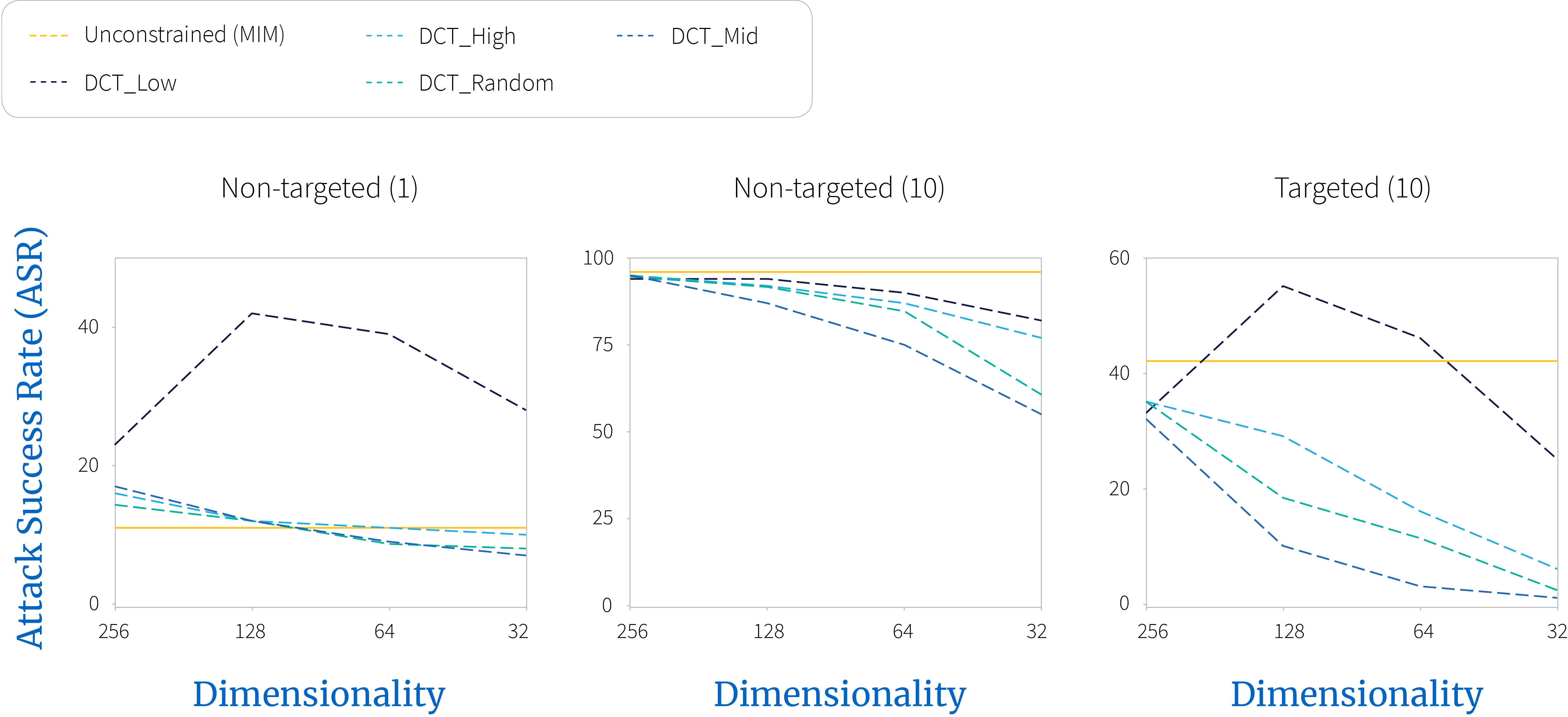
Figure 2. $\textbf{White-box}$ attack on adversarially trained model, EnsAdv. Low frequency perturbations can be generated more efficiently.
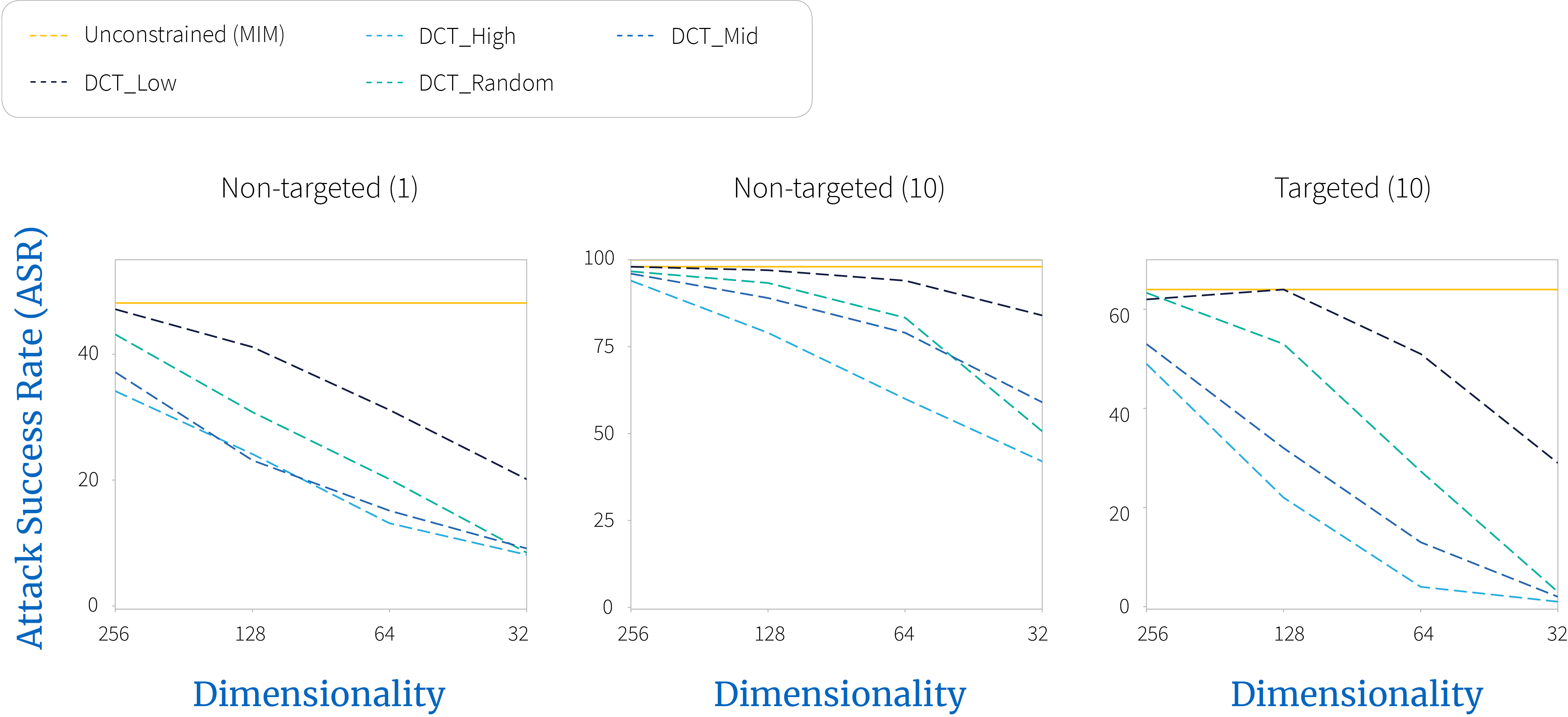
Figure 3. $\textbf{White-box}$ attack on standard undefended model, NasNet. No tangible benefit for using low frequency perturbations can be observed.
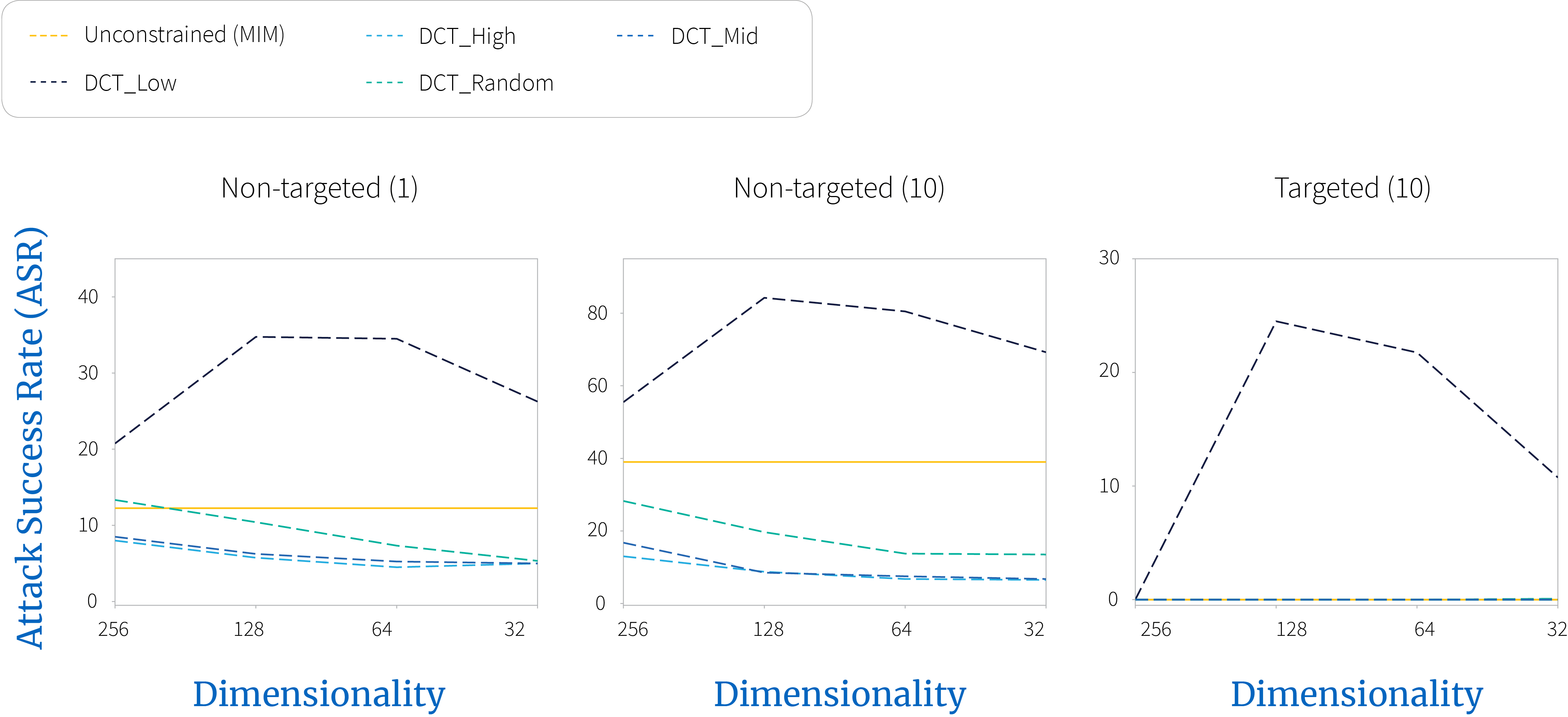
Figure 4. $\textbf{Grey-box}$ attack on top-4 NeurIPS 2017 defenses, D1$\sim$4, prepended to adversarially trained model. Clearly, low frequency perturbations appear more effective.
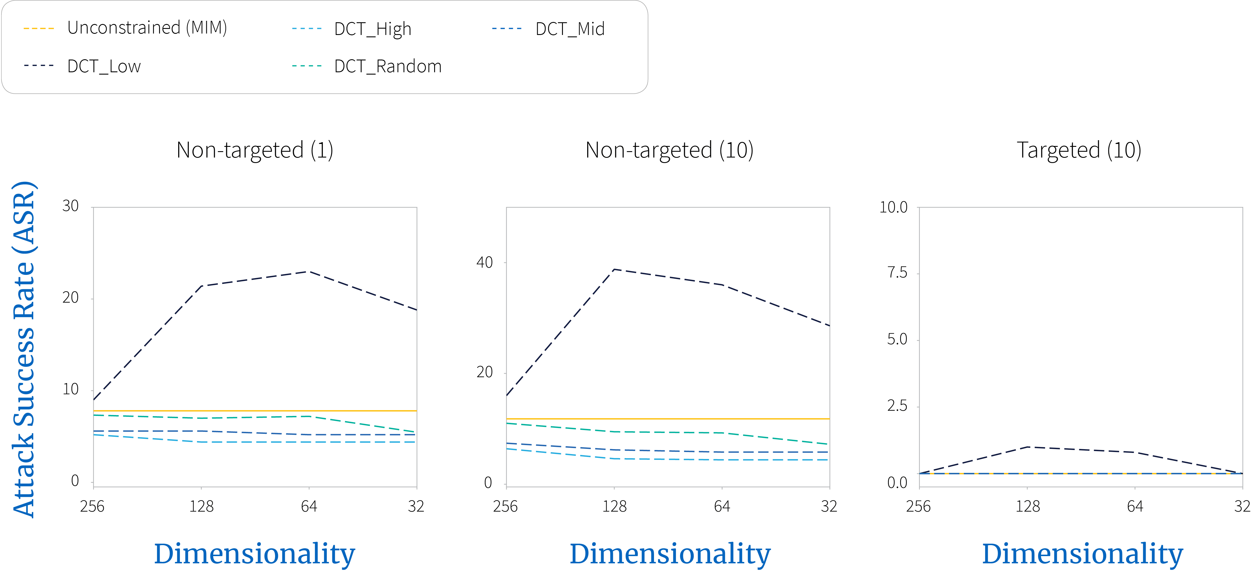
Figure 5. $\textbf{Black-box}$ attack on sources (Cln_1, Cln_3, Adv_1, Adv_3) transferred to defenses (EnsAdv + D1$\sim$4). Clearly, low frequency perturbations appear more effective.
This can be seen more clearly when tracking each individual source-target pair (figure 6). Specifically, we can see that the NeurIPS 2017 competition winners provide almost no additional robustness to the underlying model when low frequency perturbations are applied.

Figure 6. Transferability matrices with attack success rates (ASRs), comparing unconstrained (a and c) with low frequency constrained ($n=128$) MIM (b and d) in the non-targeted case. (a and b) are with $\text{iterations}=1$, (c and d) are with $\text{iterations}=10$. The column Cln is NasNet, Adv is EnsAdv. The NeurIPS 2017 competition winners provide almost no additional robustness to the underlying model when low frequency perturbations are applied.
However, we do observe that low frequency perturbations do not improve black-box transfer between undefended models. Figure 7 presents the normalized difference between attack success rate (ASR) on each of the target models with ASR on the undefended model, showing that defended models are roughly as vulnerable as undefended models when encountered by low frequency perturbations.

Figure 7. Transferability matrices with relative difference in attack success rate with the Cln model (first column). The defended models are roughly as vulnerable as undefended models when encountered by low frequency perturbations.
Discussion
Our results demonstrate that given the same search space size, only low frequency perturbations yield performance improvement, namely in generation efficiency and effectiveness when evaluated against defended ImageNet models. When confronted with low frequency perturbations, the top-4 NeurIPS 2017 defenses provide no robustness benefit, and are roughly as vulnerable as undefended models. The question remains though: does adversarially perturbing the low frequency components of the input affect human perception?
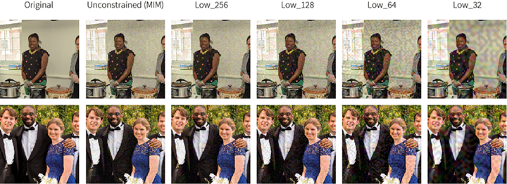
Figure 8. Adversarial examples generated with $\ell_\infty$ $\epsilon=16/255$ distortion
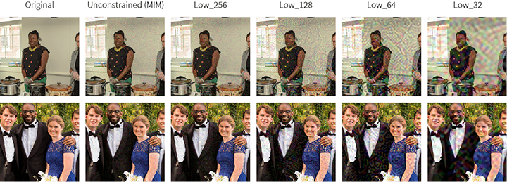
Figure 9. Adversarial examples generated with $\ell_\infty$ $\epsilon=32/255$ distortion
Representative examples are shown in figures 8 and 9. Though the perturbations do not significantly change human perceptual judgement (e.g., the top example still appears to be a standing woman), the perturbations with $n\leq 128$ are indeed perceptible. Although it is well-known that $\ell_p$-norms (in input space) are far from metrics aligned with human perception, it is still assumed that with a small enough bound (e.g. $\ell_\infty$ $\epsilon=16/255$), the resulting ball will constitute a subset of the imperceptible region (Kolter & Madry 2018). The fact that low frequency perturbations are fairly visible challenges this common belief.
In all, we hope our study encourages researchers to not only consider the frequency space, but perceptual priors in general, when bounding perturbations and proposing tractable, reliable defenses.
1https://github.com/tensorflow/models/tree/master/research/adv_imagenet_models
2https://github.com/tensorflow/models/tree/master/research/slim