It is challenging to follow all of the news and opinion about a company on social media; there are an enormous number of potentially relevant posts, and it is time-consuming to sift through them all. A recent RBC Borealis product was designed to alleviate this problem by extracting social media data in real-time, comprehend the subject matter, and provide a label for each post indicating its type. For example, a post might be tagged as “press release”, “user review” or “noise”. These labels allow users to find cleaner subsets of social media posts that they are interested in.
To build a machine learning model to classify posts into these categories, it is necessary to have high-quality labeled data for training. In other words, we need examples of social media posts that are manually labeled as press releases or user reviews to learn how to recognize new examples of the same type.
Unfortunately, manual labeling is arduous and slow. Moreover, it can be expensive if it is done by the machine learning team or if it requires domain experts. One solution is to crowdsource the labels, but this brings extra data management costs to ensure labelers are trustworthy. Third-party labeling services can handle these concerns, but bring other challenges such as losing transparency during the labeling process, slowing turnover time, and managing the restricted use of sensitive data. Turnover time and labeling effort are a particular problem in the early phases of a project; things change frequently during the ideation phase, and labelers need clear-cut instructions, not fuzzy heuristics. A change of focus can impact previously labeled data and the work must start again from nothing. The R&D process becomes a very slow-moving dance.
Fortunately, recent breakthroughs in NLP decrease this need for labeled training data. It is now typical to pre-train models by teaching them to fill in missing words in sentences. This language modeling task does not require manual labels and allows us to build models that transform the input text into a rich context-aware representation. This representation can be used as the input to our more specialized task. It reduces the need for training data because it has already learned a lot about how language works and even has some basic common sense about the world. For example, such models can correctly complete a sentence like “The train pulled up to the…” with the word “station”, so at least on a very superficial level, they can be considered to know something about rail transport.
Although these language models reduce the need for manual labeling, some high-quality labeled data is still required to train the model for the final task. In this blog, we showcase how we leveraged weak supervision to quickly iterate on product development and discuss the subsequent impact of adopting weak supervision on our workflow.
Weak supervision to the rescue
The term weak supervision refers to training machine learning models using noisy labels instead of “gold” labels in which we have high confidence. Such noisy labels, or weak labels, are generally much easier to acquire than the gold labels and can be used to train high-performing machine learning models in certain circumstances.
The Snorkel framework proposes a programmed labeling approach. Here, noisy labels are created by using easy-to-understand heuristics that come from domain knowledge of the data. For example, if a social media post contains the word “review,” then it may well be a user review. This is a good rule of thumb, but there will be plenty of cases where this word is used and the post is about something completely different, and so the output is noisy. In practice, this heuristic is applied by a short piece of code called a labeling function (LF) that takes the post and returns a label or indicates that it is uncertain by abstaining from returning a label. In this example, it might return a positive result if it sees the word “review” and indicate uncertainty if not. Other LFs might be focused on negative cases, and assign a negative label or indicate uncertainty.
A single labeling function will produce very noisy output, so several different labeling functions are used and their outputs are combined to produce a single label based on their agreement; this can be done by simple majority voting or other more involved methods. These final weak labels are then used to create training/validation and test datasets and the machine learning classifier is trained as normal.
Labeling functions can be quite powerful and offer many advantages. Take a moment to ponder the difference in scalability between manually assigning a label to a single data point, and writing a LF that assign labels to entire portions of the training set. In addition, an active learning procedure can be used to improve the assigned labels; one can manually examine datapoints where a trained model has high uncertainty in its predictive distribution and write new LFs to cover these cases.
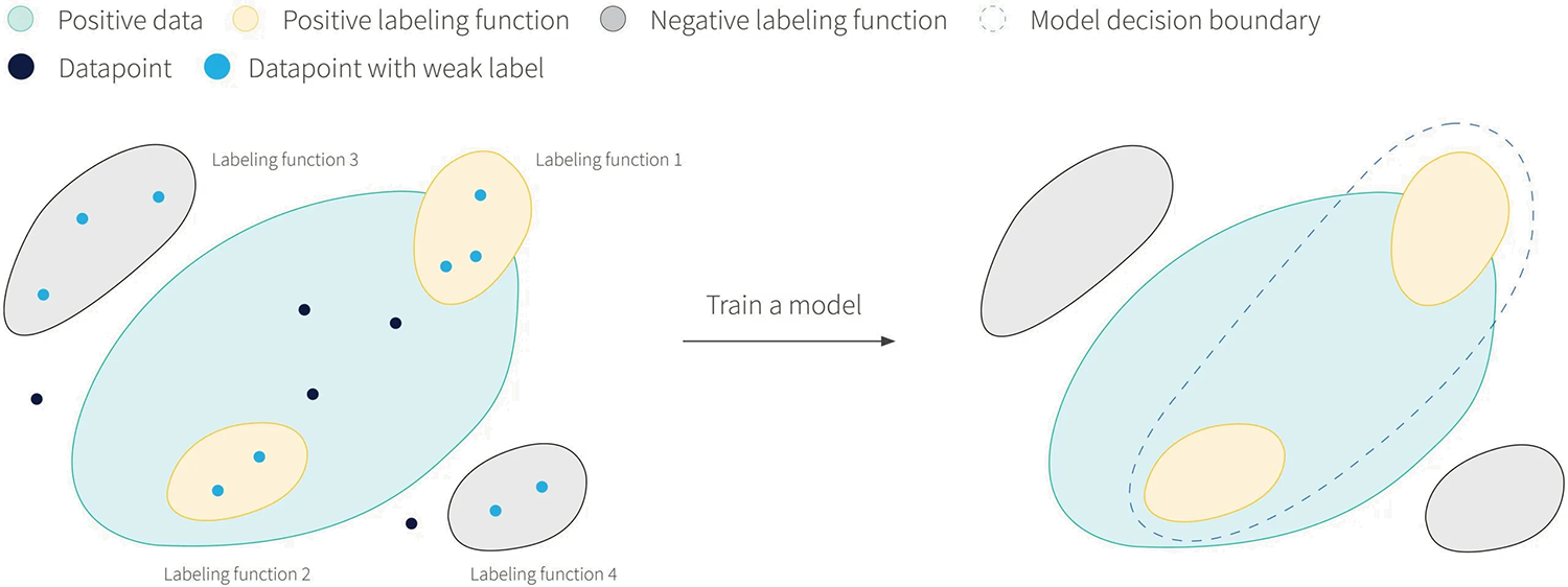
Because labeling functions don’t propose a label if they are too uncertain, it is likely that a set of LFs can only label part of the whole data space. Figure 1 shows a situation where four LFs are defined; two of these generate positive labels and two generate negative labels. Only data that fall within the regions covered by the LFs would be usable for supervised learning. However, it is possible to train a model that generalizes outside these regions through regularization techniques and through the ability of training procedures to leverage features of the data that aren’t captured by the LFs.

Figure 1: a) The true manifold for the positive class of a binary classification problem is shown in blue. Four weak labelers are defined with limited coverage: their decision boundaries are in yellow/gray and corresponds to assigning positive/negative labels. Only the subset of datapoints falling within these regions are assigned a weak label and can be used to train a model. On the right, the decision boundary of a trained model shows how generalization beyond the coverage of the LFs could manifest itself.
Another advantage of LFs is that they can be easily understood and modified. A sudden change in the definition of a class can be handled by an audit of the LFs code which can be subsequently modified to align with the new definition (see Figure 2).

Figure 2: a) Programmatic labeling allow us to quickly adapt to changing requirements. When the class definition is modified (so the blue positive region changes), we find that LF2 is now inadequate; it labels many examples outside the blue region as positive. b) In this case, we can easily modify the LF2 source code and recompute all of the weak labels.
The end result of using programmatic labeling is a transparent and deterministic pipeline that covers the ingestion of raw, unlabeled data, to a fully trained machine learning model that can be put in a production system. For our case, using this weak supervision framework on large text classification problems helped us reduce model development time from weeks to days. This allowed us to have quicker iterations with the end users which improved the product development cycle as a whole. It also enabled the validation of many ideas that would have never been prioritized due to a poor risk-reward trade-off if hand labeling was required.
New monitoring signals for free
As we deployed our trained model to production, we stumbled upon a second interesting use case for labeling functions. We can use a set of LFs to monitor the model’s performance. This was of particular interest because we were dealing with live text data streams. The dangers of domain shift (in which the distribution of input data changes) and concept drift (in which the relationship between the input data and the labels changes) are very real and detecting these phenomena quickly is challenging.
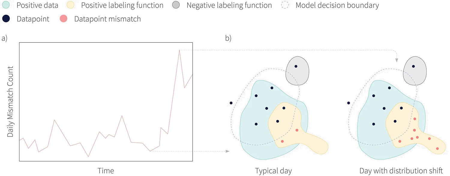
Labeling functions have different coverage than the trained model and we can exploit this fact to devise a system sensitive to these phenomena in the live data distribution. On a typical day, we expect a certain number of discrepancies between the model’s prediction and our LF’s prediction. We refer to these as mismatches. By looking at aggregated statistics, such as the daily mismatch count, a powerful time series signal is created wherein a deviation from the norm is indicative of issues with the system. In this setting, we could think of LFs as acting like smoke detectors that sounds an alarm whenever there is a change in the part of the data distribution for which they are designed to capture. Figure 3 illustrates this idea.

Figure 3: a) A time series of mismatch count between the outputs of a labeling function and the model. b) A shift in the input data distribution may cause additional mismatches which translates to a change in the expected count. When such anomalies in the time series are seen, alerts can be raised to the relevant stakeholders.
An added benefit of this system is that the LFs typically capture some domain knowledge about the data. Creating a time series signal per LF allows us to tie their anomalies to the aspect of the data for which they were designed. In one use case, we were monitoring noise filters used to clean a data stream that consisted of news about a biotech organization, and after a few months we saw a large spike in daily mismatch counts. Upon close examination we found that one of the LFs was tagging the related text snippets as noise due to a confounding acronym that appeared in the company’s recent trial results. Many more such examples were seen after the deployment of this system. Generally, we found that having this level of interpretability worked best when the LFs had high precision, and so not all the LFs were directly converted into monitoring signals; many were reworked to have less coverage (recall) but higher precision.
This monitoring system gave us the ability to insert automated checks that the deployed model was performing adequately. As such it played a big role in our confidence of the system performance and transformed alarms into actionable tasks in which the team would often uncover regions of the data distributions that our deployed model was not well trained to handle. The uncovered issues would be fixed by (re)writing new LFs and doing a full retraining.
Concluding with caution: challenges of labeling functions and the need for creativity
Writing good labeling functions is an art, not a science. Every task comes with its own quirks and challenges that can greatly impact the ease of LF creation. We found that NLP tasks are particularly well suited to the Snorkel framework due to how text data is analyzed via code (e.g., keyword-based LFs are very easily coded), and this may be large reason for the success of this application to our use cases.
Nevertheless, tackling labeling challenges is a core part of data management and the development of ML solutions. At RBC Borealis, we’ve experienced the value-add that programmatic labeling can bring, motivating us to seek out clever ways to write LFs for different types of unlabeled data. Unsurprisingly, our story is not uncommon. It will be interesting to see if these tools can eventually be exposed to business users, facilitating the adoption of machine learning into new domains and applications.