
This blog is the first in a series in which we consider machine learning from four different viewpoints. We either use gradient descent or a fully Bayesian approach, and for each, we can choose to focus on either the network weights or the output function (figure 1). To make these four viewpoints easy to understand, we first consider the linear regression model for which all four viewpoints yield tractable solutions.
This blog concerns gradient descent for which we can write closed-form expressions for the evolution of the parameters and the function itself. By analyzing these expressions, we can gain insights into the trainability and convergence speed of the model. In part II and part III, we replace the linear model with a neural network. This leads to the development of the neural tangent kernel (NTK), which provides insights into the trainability and convergence speed of neural networks.
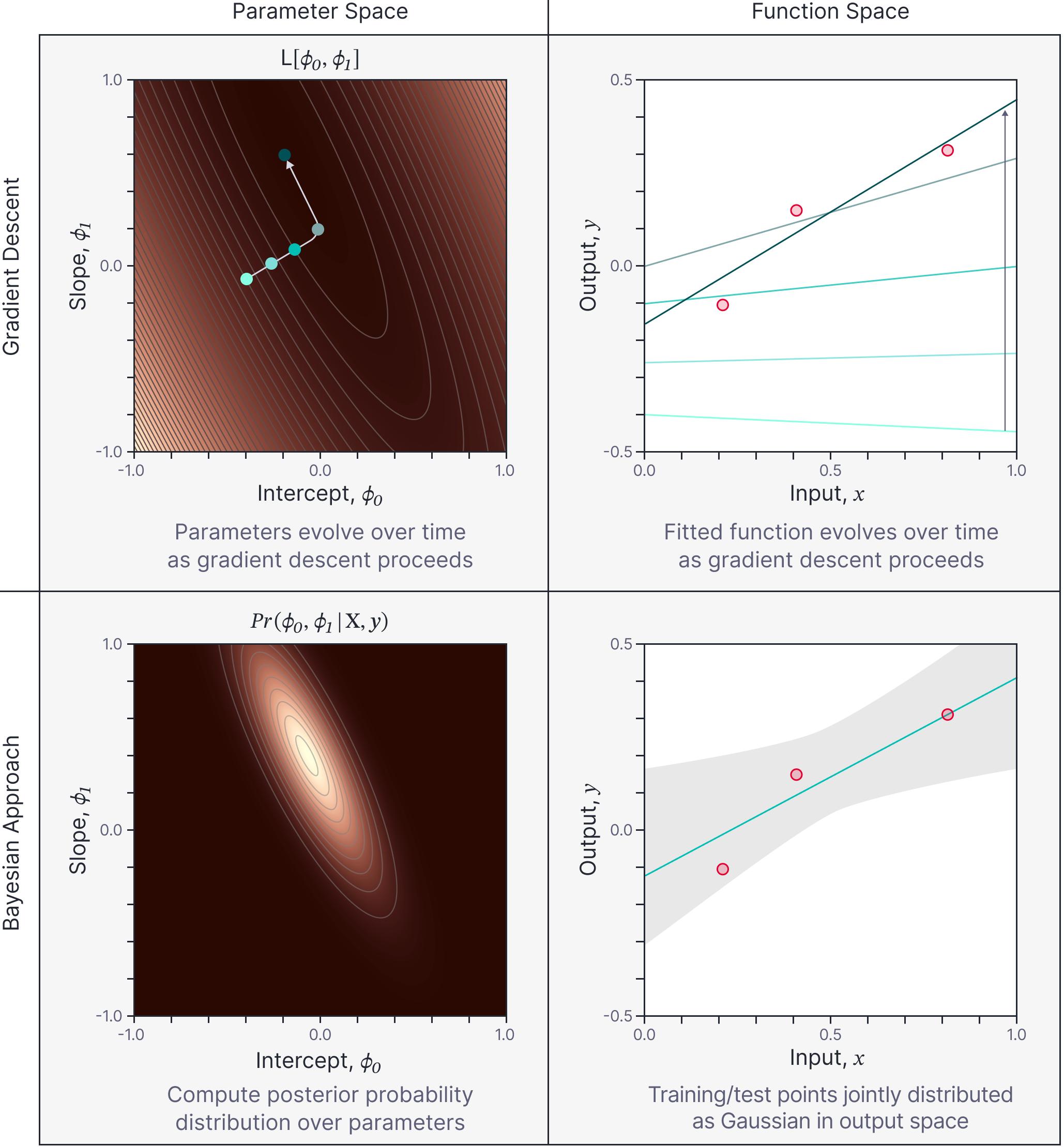
Figure 1. Four approaches to model fitting. We can either consider gradient descent (top row) or a Bayesian approach (bottom row). For either we can consider either parameter space (left column) or the function space (right column). This blog concerns the gradient descent (top row) for the linear regression model. Parts II and III of this series concerns gradient descent in neural network models which leads to the Neural Tangent Kernel (NTK). Subsequent parts concern the Bayesian approach (bottom row) for linear regression and neural networks, which leads to Bayesian neural networks (parameter space) and neural network Gaussian processes (function space). Figure inspired by $\href{https://www.youtube.com/watch?v=fcpI5z9q91A&t=1394s}{\color{blue}Sohl-Dickstein (2021).}$
In part IV and part V of this series, we consider the Bayesian approach to model fitting. We show that for the linear regression model, it is possible to derive a closed-form expression for the posterior probability over the model parameters and marginalize over this distribution to make predictions. Alternatively, we can consider the output function as a Gaussian process, and make predictions using the conditional relation for normal distributions. In parts VI and part VII, we again replace the linear regression model with a neural network and this leads to Bayesian neural networks (Bayesian approach with parameters), and neural network Gaussian processes (Bayesian approach with output function).
*The code related to this blog post can be found on github here.
Linear Regression model
A linear regression model $\mbox{f}[\mathbf{x},\boldsymbol\phi]$ computes a single scalar output:
\begin{equation}
\mbox{f}[\mathbf{x},\boldsymbol\phi] = \mathbf{x}^{T}\boldsymbol\phi,
\tag{1}
\end{equation}
where $\mathbf{x} \in\mathbb{R}^{D}$ is the input data vector and $\boldsymbol\phi\in\mathbb{R}^{D}$ are the parameters of model. We can extend this to an affine model by setting $\mathbf{x}\leftarrow [1 \quad \mathbf{x}^{T}]^{T}$ (i.e., inserting the value 1 at the start of the input vector), where now the first value of $\boldsymbol\phi$ controls the y-offset (bias) of the model. For convenience, and according to the usual convention in machine learning, we will still refer to this as a linear model.
Such a model can be trained using $I$ pairs $\{\mathbf{x}_{i},y_{i}\}$ of training data and the parameters $\hat{\boldsymbol\phi}$ are typically chosen such that they minimize the least squares loss between the model predictions $\mbox{f}[\mathbf{x}_i,\boldsymbol\phi]$ and the ground truth target values $y_{i}$:
\begin{eqnarray}
\hat{\boldsymbol\phi}= \mathop{argmin}_{\boldsymbol\phi}\Bigl[\mbox{L}[\boldsymbol\phi]\Bigr] &=&\mathop{argmin}_{\boldsymbol\phi}\left[\frac{1}{2}\sum_{i=1}^{I}\Bigl(\mbox{f}[\mathbf{x}_i,\boldsymbol\phi]-y_{i}\Bigr)^2\right]\nonumber \\
&=&\mathop{argmin}_{\boldsymbol\phi}\left[\frac{1}{2}\sum_{i=1}^{I}\Bigl(\mathbf{x}_i^T\boldsymbol\phi-y_{i}\Bigr)^2\right],
\tag{2}
\end{eqnarray}
where we have substituted in the definition of the linear model in the second line. The factor 1/2 does not change the position of the minimum but simplifies subsequent expressions.
For convenience, we will store all of the training data vectors $\{\mathbf{x}_{i}\}$ in the columns of a matrix $\mathbf{X}\in\mathbb{R}^{D\times I}$ and the targets $\{y_{i}\}$ in a column vector $\mathbf{y}\in\mathbb{R}^{I\times 1}$ and then equivalently write:
\begin{eqnarray}
\hat{\boldsymbol\phi}&=&
\mathop{argmin}_{\boldsymbol\phi}\biggl[\frac{1}{2}\Bigl(\mathbf{f}[\mathbf{X},\boldsymbol\phi] – \mathbf{y}\Bigr)^T\Bigl(\mathbf{f}[\mathbf{X},\boldsymbol\phi] – \mathbf{y}\Bigr)\biggr]\nonumber \\
&=& \mathop{argmin}_{\boldsymbol\phi}\biggl[\frac{1}{2}\Bigl(\mathbf{X}^{T}\boldsymbol\phi – \mathbf{y}\Bigr)^T\Bigl(\mathbf{X}^{T}\boldsymbol\phi – \mathbf{y}\Bigr)\biggr].
\tag{3}
\end{eqnarray}
Here, the model $\mathbf{f}[\mathbf{X},\boldsymbol\phi] = \mathbf{X}^{T}\boldsymbol\phi$ is applied to all of the data simultaneously and produces an $I\times 1$ column vector whose $i^{th}$ entry is $\mbox{f}[\mathbf{x}_i,\boldsymbol\phi]=\mathbf{x}_i^{T}\boldsymbol\phi$. Figure 2 illustrates this loss function for the case where we are fitting a line to $I=3$ data points.
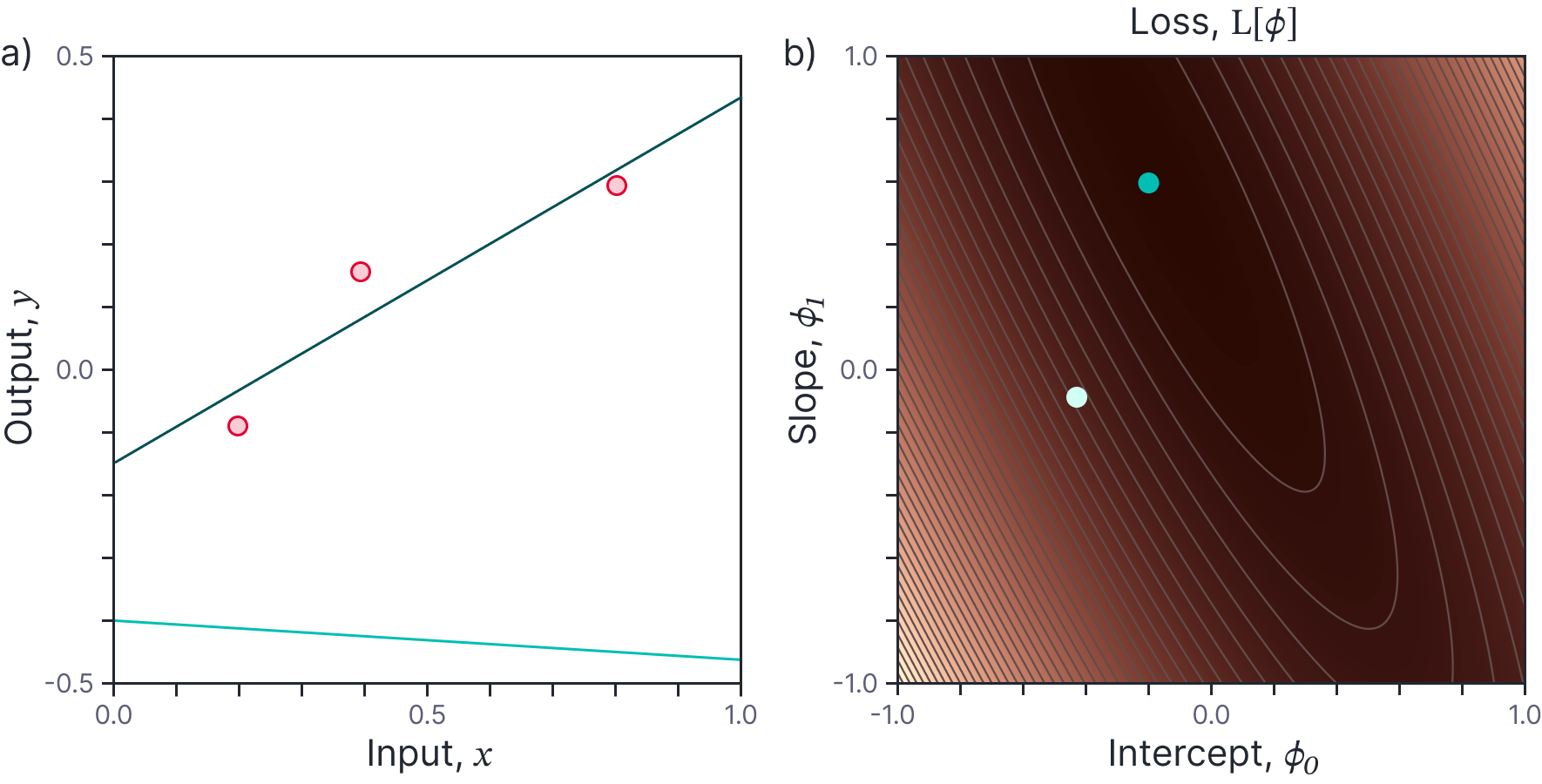
Figure 2. Loss function. a) Consider fitting a line to three points. The line is defined by two parameters: the y-intercept $\phi_{0}$ and the slope $\phi_{1}$. Two example lines shown. b) Each line (combination of parameters) results in a different loss and this can be visualized as a surface (loss indicated by brightness, gray lines are isocontours). The best fitting line corresponds to the combination of parameters that yield the lowest loss (green point).
Gradient descent and gradient flow
In gradient descent, we randomly initialize the parameters of the model to values $\boldsymbol\phi_0$. We then measure the gradient of the loss function with respect to the parameters at this point and take a step of size $\alpha$ in the downhill (negative gradient) direction. By iterating these two steps, we hope to reach the point on the loss function with minimum loss.
More formally, when we perform gradient descent, we apply the update rule:
\begin{equation}\label{eq:four_gd}
\boldsymbol\phi_{t+1} = \boldsymbol\phi_{t} – \alpha\cdot \frac{\partial L}{\partial \boldsymbol\phi}
\tag{4}
\end{equation}
where $\boldsymbol\phi_{t}$ represents the parameters at time $t$ and $\alpha$ is termed the learning rate. For the case of the linear regression model, the loss function is convex and so we are guaranteed to reach the global minimum eventually if the learning rate is sufficiently small.
Gradient flow
The above description is how we typically think about gradient descent in machine learning. However, in this blog we consider what happens when we use an infinitesimally small learning rate $\alpha$. Consider rearranging equation 4:
\begin{equation}
\frac{\boldsymbol\phi_{t+1}-\boldsymbol\phi_{t}}{\alpha} = -\frac{\partial L}{\partial \boldsymbol\phi},
\tag{5}
\end{equation}
and then letting the learning rate $\alpha$ tend zero to get:
\begin{equation}
\frac{d\boldsymbol\phi}{dt} = -\frac{\partial L}{\partial \boldsymbol\phi}.
\tag{6}
\end{equation}
This ordinary differential equation (ODE) is known as gradient flow and tells us how the parameters change over time We will see that for the linear regression model and for known initial parameters, we can solve this ODE to derive a closed-form expression for the parameter values at any given time during training.
Gradient flow for least squares loss
For the least squares loss function we can expand the right hand side of equation 6 to get the expression:
\begin{eqnarray}\label{eq:four_phi_ode}
\frac{d\boldsymbol\phi}{dt} &=& -\frac{\partial L}{\partial \boldsymbol\phi} \nonumber \\
&=& -\frac{\partial }{\partial \boldsymbol\phi}\left[\frac{1}{2} \Bigl(\mathbf {f}[\mathbf{X},\boldsymbol\phi] – \mathbf{y}\Bigr)^T\Bigl(\mathbf{f}[\mathbf{X},\boldsymbol\phi] – \mathbf{y}\Bigr)\right],
\nonumber \\
&=&
-\frac{\partial \mathbf{f}[\mathbf{X},\boldsymbol\phi]}{\partial \boldsymbol\phi}^T\bigl(\mathbf{f}[\mathbf{X},\boldsymbol\phi]-\mathbf{y}\bigr),
\tag{7}
\end{eqnarray}
where we have used the chain rule on the quadratic loss function between lines two and three.
Evolution of residual
We now consider the residual vector (i.e., the differences between the model predictions ${\bf f}[\mathbf{X},\boldsymbol\phi_t]$ and the ground truth values $\mathbf{y}$). Just as equation 7 described how the parameters evolve, it is possible to write an ODE that describes how the residual vector ${\bf f}[\mathbf{X},\boldsymbol\phi_t]-\mathbf{y}$ changes over time.
\begin{eqnarray}\label{eq:four_r_ode}
\frac{d}{dt}\Bigl[\mathbf{f}[\mathbf{X},\boldsymbol\phi]-\mathbf{y}\Bigr] &=& \frac{d \mathbf{f}[\mathbf{X},\boldsymbol\phi]}{dt}\nonumber \\ &=&\frac{\partial \mathbf{f}[\mathbf{X},\boldsymbol\phi]}{\partial \boldsymbol\phi} \frac{d\boldsymbol\phi}{dt}\nonumber \\
&=& -\left(\frac{\partial \mathbf{f}[\mathbf{X},\boldsymbol\phi]}{\partial \boldsymbol\phi} \frac{\partial \mathbf{f}[\mathbf{X},\boldsymbol\phi]}{\partial \boldsymbol\phi}^T\right)\Bigl(\mathbf{f}[\mathbf{X},\boldsymbol\phi]-\mathbf{y}\Bigr),
\tag{8}
\end{eqnarray}
where the first equality sign follows because only the first term $\mathbf{f}[\mathbf{X},\boldsymbol\phi]$ in the residual vector $\mathbf{f}[\mathbf{X},\boldsymbol\phi]-\mathbf{y}$ changes over time. The second line is an application of the chain rule, and the final expression follows from substituting in the result from equation 7.
Closed-form solution for function evolution
The ODE in equation 8 describes an exponential decay of the residual $\mathbf{f}[\mathbf{X},\boldsymbol\phi]-\mathbf{y}$. If the product of the gradients in the exponential term is constant, it has a simple solution (see this article) that is expressed in terms of the matrix exponential:
\begin{equation}
\mathbf{f}[\mathbf{X},\boldsymbol\phi_t]-\mathbf{y} = \exp\left[-\frac{\partial \mathbf{f}[\mathbf{X},\boldsymbol\phi_t]}{\partial \boldsymbol\phi} \frac{\partial \mathbf{f}[\mathbf{X},\boldsymbol\phi_t]}{\partial \boldsymbol\phi}^T\cdot t\right] \Bigl(\mathbf{f}[\mathbf{X},\boldsymbol\phi_0]-\mathbf{y}\Bigr),
\tag{9}
\end{equation}
where $\mathbf{f}[\mathbf{X},\boldsymbol\phi_0]-\mathbf{y}$ is the initial residual vector that contains to the signed errors with the initial parameters $\boldsymbol\phi_{0}$. When $t=0$, it can be verified that both the left and right sides correspond to this initial vector.
Rearranging, this equation, we can get a closed-form solution for the evolution of the function $\mathbf{f}[\mathbf{X},\boldsymbol\phi_t]$ at the training points $\mathbf{X}$:
\begin{eqnarray}
\mathbf{f}[\mathbf{X},\boldsymbol\phi_t] &=& \mathbf{y} + \exp\left[-\frac{\partial \mathbf{f}[\mathbf{X},\boldsymbol\phi_t]}{\partial \boldsymbol\phi} \frac{\partial \mathbf{f}[\mathbf{X},\boldsymbol\phi_t]}{\partial \boldsymbol\phi}^T\cdot t\right] \Bigl(\mathbf{f}[\mathbf{X},\boldsymbol\phi_0]-\mathbf{y}\Bigr).
\tag{10}
\end{eqnarray}
This tells us how the function at the data points evolves as gradient descent proceeds. By analyzing these expressions we can get information about the trainability of the model (i.e., the ability of the model to fit the training data exactly) as well as the convergence speed of the training process (i.e., how fast this happens).
Trainability and convergence in the linear model
Let’s examine the implications of this expression for the linear model for which:
\begin{eqnarray}
\mathbf{f}[\mathbf{X},\boldsymbol\phi_t] &=& \mathbf{X}^{T}\boldsymbol\phi_t\nonumber \\
\frac{\partial \mathbf{f}[\mathbf{X},\boldsymbol\phi_t]}{\partial \boldsymbol\phi_t} &=& \mathbf{X}^T.
\tag{11}
\end{eqnarray}
In this case the derivative does not depend on the current parameters $\boldsymbol\phi_t$. Substituting these expressions into equation 10 yields:
\begin{eqnarray}
\mathbf{f}[\mathbf{X},\boldsymbol\phi_t] &=& \mathbf{y} + \exp\left[-\mathbf{X}^{T}\mathbf{X}\cdot t\right] \Bigl(\mathbf{X}^{T}\boldsymbol\phi_0-\mathbf{y}\Bigr).
\tag{12}
\end{eqnarray}
The evolution of this function is depicted in figure 3.
Figure 3. Function evolution for linear model. a) Consider fitting a line, starting at initial parameters $\boldsymbol\phi_0$ (cyan line) and using gradient descent to find the best parameters (green line). b) Equation 12 describes how the model predictions at the three training points evolve over time towards their final values. c) We can also examine how the residuals (discrepancy between model prediction and ground truth) evolve over time.
Trainability: We can draw conclusions about the trainability of the model by examining the exponential term in equation 12.
- If $\mathbf{X}^T\mathbf{X}$ is full rank, then the exponential term will become zero when $t\rightarrow \infty$ and the function $\mathbf{f}[\mathbf{X},\boldsymbol\phi_t]$ will fit the prediction $\mathbf{y}$ exactly.
- Conversely, if the matrix $\mathbf{X}^T\mathbf{X}$ it is not full rank, the function will not fit the prediction exactly. The residual errors depend on the null space of $\mathbf{X}^T\mathbf{X}$.
This aligns with our expectations. The data matrix $\mathbf{X}$ has size $(D+1)\times I$ where $D$ is the input data dimension (recall that we appended a 1 to each data example). Hence, the matrix $\mathbf{X}^T\mathbf{X}$ will be full rank if $I\leq D+1$ (i.e., if the number of data points is less than or equal to the number of parameters). For the case, of fitting a line there are $D+1=2$ parameters and we can fit $I=1$ or $I=2$ points exactly. However, a line cannot pass exactly through $I> 2$ data points in general position.
Convergence speed: Equation 12 can also tell us about the speed of convergence. The time taken to converge depends on the (i) the eigenvalues of $\mathbf{X}^{T}\mathbf{X}$ (which tell us how fast the function changes) and (ii) the magnitude of the initial error $\mathbf{X}^{T}\boldsymbol\phi_0-\mathbf{y}$ when projected onto the corresponding eigenvectors (which tells us how far we need to change). Discarding the second of these quantities (which depends on the particular initialization), we can loosely say that the time to converge depends on the smallest eigenvalue of $\mathbf{X}^{T}\mathbf{X}$.
These results are perhaps not surprising for the the linear regression model, but in part II of this series, we’ll apply the same ideas to gain insight into the trainability and convergence of neural networks.
Evolution of parameters
Let’s assume that the model is close to linear. In this case, it is well approximated by retaining only the linear term from a Taylor expansion around the initial parameters $\boldsymbol\phi_0$:
\begin{equation}
\mathbf{f}[\mathbf{X},\boldsymbol\phi_t] \approx \mathbf{f}[\mathbf{X},\boldsymbol\phi_0] + \frac{\partial \mathbf{f}[\mathbf{X},\boldsymbol\phi_0]}{\partial \boldsymbol\phi}\bigl(\boldsymbol\phi_t-\boldsymbol\phi_{0}\bigr)
\tag{13}
\end{equation}
We replace the left hand side of equation 10 with this expression to yield:
\begin{eqnarray}
\mathbf{f}[\mathbf{X},\boldsymbol\phi_0] + \frac{\partial \mathbf{f}[\mathbf{X},\boldsymbol\phi_0]}{\partial \boldsymbol\phi}\bigl(\boldsymbol\phi_t-\boldsymbol\phi_{0}\bigr) &&\tag{14} \\ &&\hspace{-3cm}=\mathbf{y} + \exp\left[-\frac{\partial \mathbf{f}[\mathbf{X},\boldsymbol\phi_t]}{\partial \boldsymbol\phi} \frac{\partial \mathbf{f}[\mathbf{X},\boldsymbol\phi_t]}{\partial \boldsymbol\phi}^T\cdot t\right] \Bigl(\mathbf{f}[\mathbf{X},\boldsymbol\phi_0]-\mathbf{y}\Bigr).
\end{eqnarray}
Moving the first term to the right-hand side, we get:
\begin{eqnarray}
\frac{\partial \mathbf{f}[\mathbf{X},\boldsymbol\phi_0]}{\partial \boldsymbol\phi}\bigl(\boldsymbol\phi_t-\boldsymbol\phi_{0}\bigr) &&\tag{15}\\
&&\hspace{-3cm}= -\left(\mathbf{I}-\exp\left[-\frac{\partial \mathbf{f}[\mathbf{X},\boldsymbol\phi_t]}{\partial \boldsymbol\phi} \frac{\partial \mathbf{f}[\mathbf{X},\boldsymbol\phi_t]}{\partial \boldsymbol\phi}^T\cdot t\right]\right) \Bigl(\mathbf{f}[\mathbf{X},\boldsymbol\phi_0]-\mathbf{y}\Bigr).
\end{eqnarray}
Finally, we can solve for $\boldsymbol\phi_{t}$:
\begin{eqnarray}
\boldsymbol\phi_t&=&\boldsymbol\phi_0 – \frac{\partial \mathbf{f}[\mathbf{X},\boldsymbol\phi_0]}{\partial \boldsymbol\phi}^+ \left(\mathbf{I}-\exp\left[-\frac{\partial \mathbf{f}[\mathbf{X},\boldsymbol\phi_t]}{\partial \boldsymbol\phi} \frac{\partial \mathbf{f}[\mathbf{X},\boldsymbol\phi_t]}{\partial \boldsymbol\phi}^T\cdot t\right]\right) \Bigl(\mathbf{f}[\mathbf{X},\boldsymbol\phi_0]-\mathbf{y}\Bigr),\tag{16} \\
\end{eqnarray}
where $\mathbf{A}^+$ denotes the Moore-Penrose pseudoinverse of $\mathbf{A}$. When the the system is overdetermined ($\mathbf{A}$ is portrait), this is given by $\mathbf{A}^+=(\mathbf{A}^{T}\mathbf{A})^{-1}\mathbf{A}^{T}$. For the underdetermined case ($\mathbf{A}$ is landscape), this is given by $\mathbf{A}^+=\mathbf{A}^T(\mathbf{A}\mathbf{A}^T)^{-1}$.
Parameter evolution for linear model
Let’s examine parameter evolution for the linear model, where:
\begin{eqnarray}
\mathbf{f}[\mathbf{X},\boldsymbol\phi_t] &=& \mathbf{X}^{T}\boldsymbol\phi_t\nonumber \\
\frac{\partial \mathbf{f}[\mathbf{X},\boldsymbol\phi_t]}{\partial \boldsymbol\phi_t} &=& \mathbf{X}^T.
\tag{17}
\end{eqnarray}
Here, the linear approximation is certainly valid (since the second derivatives are zero). Substituting these expressions into equation 16 for the overdetermined case, we get:
\begin{eqnarray}
\boldsymbol\phi_t &=&\boldsymbol\phi_0 -(\mathbf{X}\mathbf{X}^{T})^{-1}\mathbf{X}\left(\mathbf{I}-\exp\left[-\mathbf{X}^{T}\mathbf{X}\cdot t\right]\right) \Bigl(\mathbf{X}^T\boldsymbol\phi_0-\mathbf{y}\Bigr).
\tag{18}
\end{eqnarray}
Figure 4 plots the evolution of the parameters for the fitting a line to the three points from figure 2.

Figure 4. Parameter evolution for fitting line to three points. a) Equation 18 shows how the parameters evolve on the loss function from their initial values $\boldsymbol\phi_0$ (cyan position) to the final values $\boldsymbol\phi_{\infty}$ (green point) at the minimum of the function. b) We can also observe how each parameter changes individually as a function of time. c) Finally, we can plot the loss function as a function of time. In this case, the loss function decreases very quickly as we descend to the valley in panel (a), and then much more slowly as we move along the valley floor.
Comparison to closed-form solution
For the linear model, it is possible to compute the least squares solution for the parameters in closed form (see end of blog for proof) using the relation:
\begin{eqnarray}
\boldsymbol\phi = (\mathbf{X}\mathbf{X}^{T})^{-1}\mathbf{X}\mathbf{y}.
\tag{19}
\end{eqnarray}
If the closed-form solution for the parameter evolution in equation 18 is correct, then we should retrieve this expression when $t\rightarrow \infty$. To see that this is true, we re-arrange equation 18 into two terms:
\begin{eqnarray}
\boldsymbol\phi_t &=&\boldsymbol\phi_0 -(\mathbf{X}\mathbf{X}^{T})^{-1}\mathbf{X}\left(\mathbf{I}-\exp\left[-\mathbf{X}^{T}\mathbf{X}\cdot t\right]\right) \Bigl(\mathbf{X}^T\boldsymbol\phi_0-\mathbf{y}\Bigr)\nonumber \\
&=& \boldsymbol\phi_0-(\mathbf{X}\mathbf{X}^{T})^{-1}(\mathbf{X}\mathbf{X}^{T}\boldsymbol\phi_0-\mathbf{X}\mathbf{y}) + (\mathbf{X}\mathbf{X}^{T})^{-1}\mathbf{X}\exp\left[-\mathbf{X}^{T}\mathbf{X}\cdot t\right] \Bigl(\mathbf{X}^T\boldsymbol\phi_0-\mathbf{y}\Bigr)\nonumber \\
&=& \boldsymbol\phi_0-(\boldsymbol\phi_0-(\mathbf{X}\mathbf{X}^{T})^{-1})\mathbf{X}\mathbf{y}) +(\mathbf{X}\mathbf{X}^{T})^{-1}\mathbf{X} \exp\left[-\mathbf{X}^{T}\mathbf{X}\cdot t\right] \Bigl(\mathbf{X}^T\boldsymbol\phi_0-\mathbf{y}\Bigr)\nonumber \\
&=& (\mathbf{X}\mathbf{X}^{T})^{-1}\mathbf{X}\mathbf{y} +(\mathbf{X}\mathbf{X}^{T})^{-1}\mathbf{X}\exp\left[-\mathbf{X}^{T}\mathbf{X}\cdot t\right] \Bigl(\mathbf{X}^T\boldsymbol\phi_0-\mathbf{y}\Bigr),
\tag{20}
\end{eqnarray}
where we have separated out the two terms from the inner bracket in line two and simplified the first of these terms in the subsequent lines.
The first term is the same as the closed-form solution, so if the second term becomes zero as $t\rightarrow \infty$, the two expressions agree. However, it’s not obvious this is the case. When there are more training points than parameters (the matrix $\mathbf{X}$ is landscape), $\mathbf{X}\mathbf{X}^{T}$ is full rank and a closed-form expression exists. However, this means that the term $\mathbf{X}^T\mathbf{X}$ in the exponential is not full rank and only part of the subspace tends to zero as $t\rightarrow \infty$. Fortunately, the part that does not tend to zero is the null space of $\mathbf{X}$, which is removed by the pre-multiplication by $\mathbf{X}$. It follows that the term $\mathbf{X}\exp\left[-\mathbf{X}^{T}\mathbf{X}\cdot t\right]$ becomes zero when $t$ becomes large, and hence:
\begin{eqnarray}
\boldsymbol\phi_\infty &=& (\mathbf{X}\mathbf{X}^{T})^{-1}\mathbf{X}\mathbf{y},
\tag{21}
\end{eqnarray}
as required.
Evolution of model predictions
Equation 18 provides a closed-form solution for the evolution of the parameters $\boldsymbol\phi_t$ over time. It follows that we can also get a closed-form solution for the evolution of the model predictions $y^* =\mbox{f}[\mathbf{x}^*,\boldsymbol\phi_{t}]$ for a new points $\mathbf{x}^*$ by passing the solution for the parameters into the model.
For the linear model, the prediction for a new point $\mathbf{x}^{*}$ is given by $y^* = \mathbf{x}^{*T}\boldsymbol\phi$, which gives the solution:
\begin{eqnarray}
y^*_{t} &=& \mathbf{x}^{*T}\boldsymbol\phi_0 -\mathbf{x}^{*T}(\mathbf{X}\mathbf{X}^{T})^{-1}\mathbf{X}\left(\mathbf{I}-\exp\left[-\mathbf{X}^{T}\mathbf{X}\cdot t\right]\right) \Bigl(\mathbf{X}^T\boldsymbol\phi_0-\mathbf{y}\Bigr),
\tag{22}
\end{eqnarray}
and when $t\rightarrow \infty$, the final predictions are given by:
\begin{equation}
\hat{y}^*= \mathbf{x}^{*T}\Bigl(\mathbf{X}\mathbf{X}^T\Bigr)^{-1}\mathbf{X}\mathbf{y}.
\tag{23}
\end{equation}
The evolution of the function for the linear model is illustrated in figure 5.

Figure 5. Evolution of predictions for fitting line to three points. For any time $t$ in the training procedure, we can get a closed-form expression for the prediction $y^*$ corresponding to a new input $x^{*}$ in terms of the training data $\{\mathbf{X},\mathbf{y}\}$ (equation 22). a) Predictions (cyan line) before training. b-e) Updated predictions during training. f) Predictions for large $t$ where training procedure has almost converged.
Evolution of prediction covariance
Finally, we note that the evolution of the predictions $y^{*}_t$ for a new point $\mathbf{x}^*$ can be written as an affine transformation of the initial parameters $\bf{\phi_{0}}$:
\begin{eqnarray}
y^*_{t} &=& \mathbf{x}^{*T}\boldsymbol\phi_0 -\mathbf{x}^{*T}(\mathbf{X}\mathbf{X}^{T})^{-1}\mathbf{X}\left(\mathbf{I}-\exp\left[-\mathbf{X}^{T}\mathbf{X}\cdot t\right]\right) \Bigl(\mathbf{X}^{T}\boldsymbol\phi_0-\mathbf{y}\Bigr)\nonumber\\
&=& \mathbf{x}^{*T}(\mathbf{X}\mathbf{X}^{T})^{-1}\mathbf{X}\left(\mathbf{I}-\exp\left[-\mathbf{X}^{T}\mathbf{X}\cdot t\right]\right)\mathbf{y} \nonumber \\
&& +\Bigl[ \hspace{1mm} 1,-\mathbf{x}^{*T}(\mathbf{X}\mathbf{X}^{T})^{-1}\mathbf{X}\left(\mathbf{I}-\exp\left[-\mathbf{X}^{T}\mathbf{X}\cdot t\right]\right)\Bigr]\begin{bmatrix}\mathbf{x}^{T*}\\ \mathbf{X}^{T}\end{bmatrix}\boldsymbol\phi_{0}\nonumber \\
&=& a +\mathbf{b}\phi_{0},
\tag{24}
\end{eqnarray}
where we have denoted the two components of the affine transform by the scalar $a$ and the row vector $\mathbf{b}$.
Now let’s define a normally distributed prior over the initial parameters $\boldsymbol\phi_0$:
\begin{equation}
Pr(\boldsymbol\phi_0) = \mbox{Norm}\Bigl[\mathbf{0}, \sigma_p^2 \mathbf{I}\Bigr],
\tag{25}
\end{equation}
with mean zero and spherical covariance $\sigma_p^2 \mathbf{I}$. The normally distributed prior implies a distribution over the initial model outputs. Because the prior distribution is normal and the transformation of the prior is affine, we can use the relation (see proof at end of blog) that if $Pr(\mathbf{z})= \mbox{Norm}_{\mathbf{z}}[\boldsymbol\mu, \boldsymbol\Sigma]$, then the affine transform $\mathbf{a}+\mathbf{B}\mathbf{z}$ is distributed as:
\begin{equation}
Pr(\mathbf{a}+\mathbf{B}\mathbf{z}) = \mbox{Norm}\Bigl[\mathbf{a} + \mathbf{B} \boldsymbol\mu, \mathbf{B}\boldsymbol\Sigma\mathbf{B}^{T}\Bigr].
\tag{26}
\end{equation}
and so can compute the mean and variance of the distribution $Pr(y_t^*)$ over the predictions as training proceeds. In practice, it is typical to add a value $\sigma^2$ to the variance to account for noise in training data. This is illustrated in figure 6.
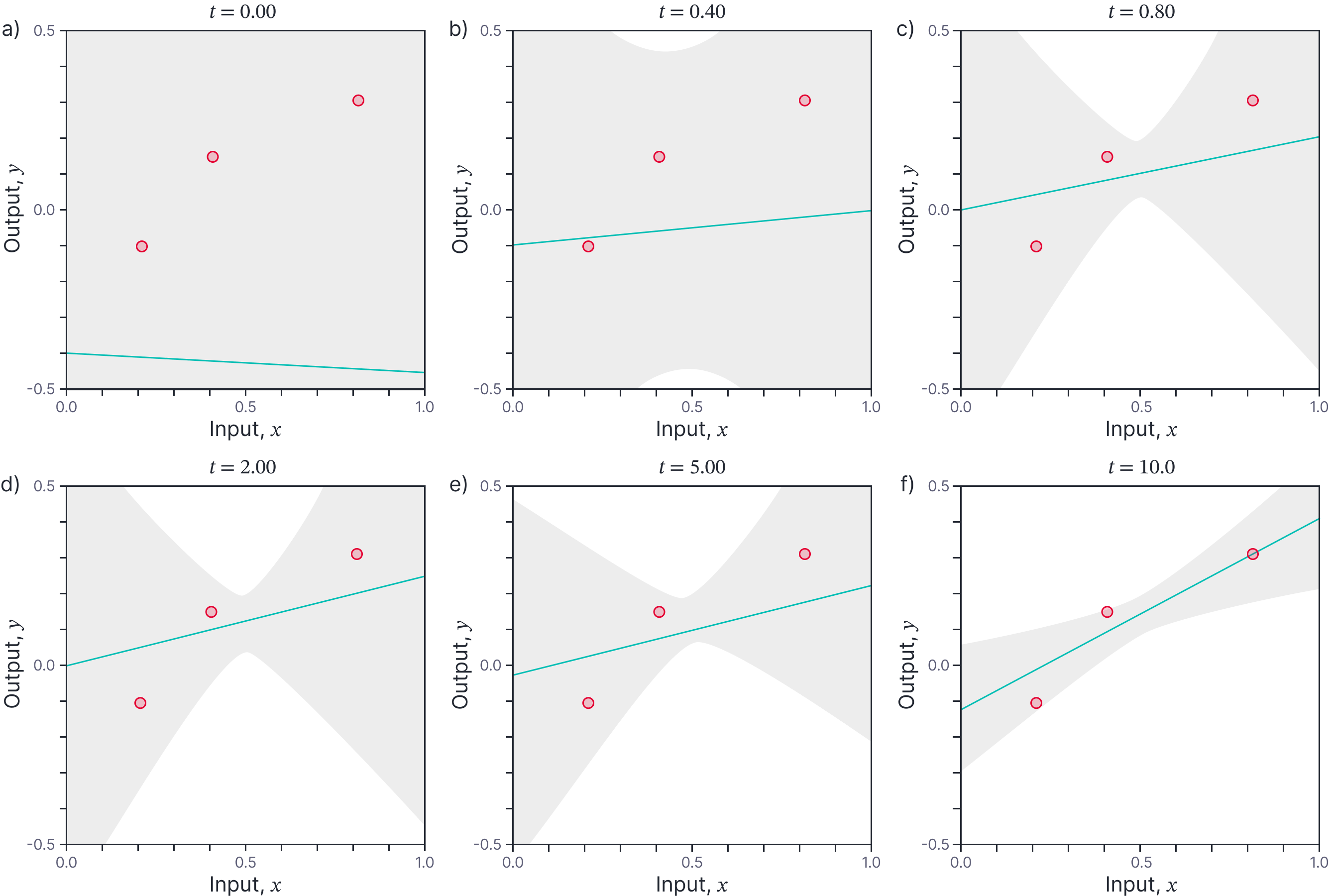
Figure 6. Evolution of predictions over time with errors. In this experiment, we assume that the prior variance $\sigma^2_p$ is $3.0$ and the noise variance $\sigma^2$ is 0.0025. At the start of training, the most likely prediction has slope and intercept of zero and the uncertainty (gray region represents $\pm 1$ standard deviation) is very high. As training proceeds, the most likely prediction fits the training data better and the variance decreases.
*The code related to this blog post can be found on GitHub here.
Discussion
This blog has considered gradient descent training using gradient flow, using linear regression as a working example. The main results are that:
- We can write a closed-form solution for the evolution of the function output at the training data points. By analyzing this solution, we can learn about the ability of the model to fit the dataset perfectly, and the speed of convergence.
- We can write a closed-form solution for the evolution of the parameters over time, which agrees with the least squares solution when $t\rightarrow \infty$.
- We can write a closed-form solution for the evolution of the predictions of the model as a function of time.
- By defining a prior over the parameters, we can also model the evolution of the uncertainty of our predictions.
In the next part of this series, we’ll develop the neural tangent kernel by applying these same ideas to a neural network model.
*The code related to this blog post can be found on github here.
Least squares solution for linear model
For a linear model, it is possible to find the final parameters in closed form. Writing out the loss function $L[\boldsymbol\phi]$ explicitly, we have:
\begin{eqnarray*}
L[\boldsymbol\phi] &=& \Bigl(\mathbf{X}^{T}\boldsymbol\phi – \mathbf{y}\Bigr)^T\Bigl(\mathbf{X}^{T}\boldsymbol\phi – \mathbf{y}\Bigr)\nonumber \\
&=& \boldsymbol\phi^{T}\mathbf{X}\mathbf{X}^{T}\boldsymbol\phi – \boldsymbol\phi^{T}\mathbf{X}\mathbf{y} -\mathbf{y}^{T}\mathbf{X}^{T}\boldsymbol\phi – \mathbf{y}^{T}\mathbf{y} \nonumber \\
&=& \boldsymbol\phi^{T}\mathbf{X}\mathbf{X}^{T}\boldsymbol\phi – 2\boldsymbol\phi^{T}\mathbf{X}\mathbf{y} – \mathbf{y}^{T}\mathbf{y},
\end{eqnarray*}
where we have expanded out terms in the second line. We note that the second and third terms are both scalars and so are equal to their own transposes and these are combined into a single term in the third line.
We can find a closed-form solution for the best parameters by computing the derivative $dL/d\boldsymbol\phi$ of the scalar loss $L$ with respect to the parameter vector $\boldsymbol\phi$, setting the result to zero:
\begin{equation*}
2\mathbf{X}\mathbf{X}^{T}\boldsymbol\phi – 2\mathbf{X}\mathbf{y} = 0
\end{equation*}
which can be rearranged to find a solution for the best parameters $\boldsymbol\phi$.
\begin{equation*}
\hat{\boldsymbol\phi}= \Bigl(\mathbf{X}\mathbf{X}^T\Bigr)^{-1}\mathbf{X}\mathbf{y}.
\end{equation*}
This result can only be computed if there are at least as many columns $I$ in $\mathbf{X}$ as there are unknown parameters $D+1$ in $\mathbf{\boldsymbol\phi}$. Otherwise, the matrix $\mathbf{A}^{T}\mathbf{A}$ will be singular. In cases like this (e.g., trying to fit a line with $D+1=2$ parameters to $I=1$ data points) the solution is ambiguous.
Affine transformations of normal distributions
The multivariate normal distribution is defined as:
\begin{equation*}
Pr(\mathbf{x}) = \frac{1}{(2\pi)^{D}|\boldsymbol\Sigma|^{1/2}}\exp\biggl[-0.5\left(\mathbf{x}-\boldsymbol\mu\right)\boldsymbol\Sigma^{-1}\left(\mathbf{x}-\boldsymbol\mu\right)\biggr].
\end{equation*}
To transform the distribution as $\mathbf{y} = \mathbf{Ax}+\mathbf{b}$, we substitute in $\mathbf{x} = \mathbf{A}^{-1}(\mathbf{y}-\mathbf{b})$ and divide by the determinant of the Jacobian of the transformation, which for this case is just $|\mathbf{A}|$ giving:
\begin{equation*}
Pr(\mathbf{x}) = \frac{1}{(2\pi)^{D}|\boldsymbol\Sigma|^{1/2}|\mathbf{A}|}\exp\biggl[-0.5\left( \mathbf{A}^{-1}(\mathbf{y}-\mathbf{b})-\boldsymbol\mu\right)\boldsymbol\Sigma^{-1}\left( \mathbf{A}^{-1}(\mathbf{y}-\mathbf{b})-\boldsymbol\mu\right)\biggr].
\end{equation*}
We’ll first work with the constant $\kappa$ from outside the exponential to show that it is the constant for a distribution with variance $\mathbf{A}\boldsymbol\Sigma\mathbf{A}^{T}$. We have:
\begin{eqnarray*}
\kappa &=& \frac{1}{(2\pi)^{D}|\boldsymbol\Sigma|^{1/2}|\mathbf{A}|}\\
&=& \frac{1}{(2\pi)^{D}|\boldsymbol\Sigma|^{1/2} |\mathbf{A}|^{1/2}|\mathbf{A}|^{1/2} }\\
&=& \frac{1}{(2\pi)^{D}|\boldsymbol\Sigma|^{1/2} |\mathbf{A}|^{1/2}|\mathbf{A}^{T}|^{1/2} }\\
&=& \frac{1}{(2\pi)^{D} |\mathbf{A}|^{1/2}|\boldsymbol\Sigma|^{1/2}|\mathbf{A}^{T}|^{1/2} }\\
&=& \frac{1}{(2\pi)^{D}|\mathbf{A}\boldsymbol\Sigma\mathbf{A}^{T}|^{1/2}},
\end{eqnarray*}
which is exactly the required constant.
Now we’ll work with the quadratic in the exponential term to show that it corresponds to a normal distribution in $\mathbf{y}$ with variance $\mathbf{A}\boldsymbol\Sigma\mathbf{A}^{T}$ and mean $\mathbf{A}\boldsymbol\mu+\mathbf{b}$.
\begin{eqnarray*}
&&\hspace{-1cm} \left( \mathbf{A}^{-1}(\mathbf{y}-\mathbf{b})-\boldsymbol\mu\right)\boldsymbol\Sigma^{-1}\left( \mathbf{A}^{-1}(\mathbf{y}-\mathbf{b})-\boldsymbol\mu\right) \\
&\!\!=\!\!&\!\!
\mathbf{y}^{T}\mathbf{A}^{-T}\boldsymbol\Sigma^{-1}\mathbf{A}^{-1}\mathbf{y} -2(\mathbf{b}^{T}\mathbf{A}^{-T}+\boldsymbol\mu^{T})\boldsymbol\Sigma^{-1}\mathbf{A}^{-1}\mathbf{y} + (\mathbf{A}^{-1}\mathbf{b}+\boldsymbol\mu)^{T}\boldsymbol\Sigma^{-1}(\mathbf{A}^{-1}\mathbf{b}+\boldsymbol\mu)\\
&\!\!=\!\!&\!\!
\mathbf{y}^{T}\mathbf{A}^{-T}\boldsymbol\Sigma^{-1}\mathbf{A}^{-1}\mathbf{y} -2(\mathbf{b}^{T}+\boldsymbol\mu^{T}\mathbf{A}^{T})\mathbf{A}^{-T}\boldsymbol\Sigma^{-1}\mathbf{A}^{-1}\mathbf{y}\\
&&\hspace{3cm} + (\mathbf{A}^{-1}\mathbf{b}+\mathbf{A}\boldsymbol\mu)^{T}\mathbf{A}^{-T}\boldsymbol\Sigma^{-1}\mathbf{A}^{-1}(\mathbf{b}+\mathbf{A}\boldsymbol\mu)\\
&\!\!=\!\!&\!\!
\left(\mathbf{y}-(\mathbf{A}\boldsymbol\mu+\mathbf{b})\right)^{T} \left(\mathbf{A}\boldsymbol\Sigma\mathbf{A}^{T}\right)^{-1}\left(\mathbf{y}-(\mathbf{A}\boldsymbol\mu+\mathbf{b})\right).
\end{eqnarray*}
This is clearly the quadratic term from a normal distribution in $\mathbf{y}$ with variance $\mathbf{A}\boldsymbol\Sigma\mathbf{A}^{T}$ and mean $\mathbf{A}\boldsymbol\mu+\mathbf{b}$ as required.
Thanks to Lechao Xiao who explained the evolution of the parameters to me.
Careers
Artificial Intelligence is reshaping finance. Every day, our teams uncover new opportunities that advance the field of AI, building products that impact millions of people across Canada and beyond. Explore open roles!
Explore opportunities