In July the Thirty-seventh International Conference on Machine Learning (ICML) was held featuring over 1,000 papers and an array of tutorials, workshops, invited talks and more. Borealis researchers were (virtually) there presenting their work
- Evaluating Lossy Compression Rates of Deep Generative Models by Sicong Huang, Alireza Makhzani, Yanshuai Cao and Roger Grosse
- On Variational Learning of Controllable Representations for Text without Supervision by Peng Xu, Jackie CK Cheung, Yanshuai Cao
- Tails of Lipschitz Triangular Flows by Priyank Jaini, Ivan Kobyzev, Yaoliang Yu and Marcus A. Brubaker
and many members of the research team took the time to virtually attend ICML 2020. Now that the conference content is freely available online, it’s a great time to look back and check out some of the highlights. In this post, four RBC Borealis researchers describe the papers that they found most interesting or significant from the conference.
Improving Generalization by Controlling Label-Noise Information in Neural Network Weights
Hrayr Harutyunyan, Kyle Reing, Greg Ver Steeg, Aram Galstyan by Peng Xu
Related Papers:

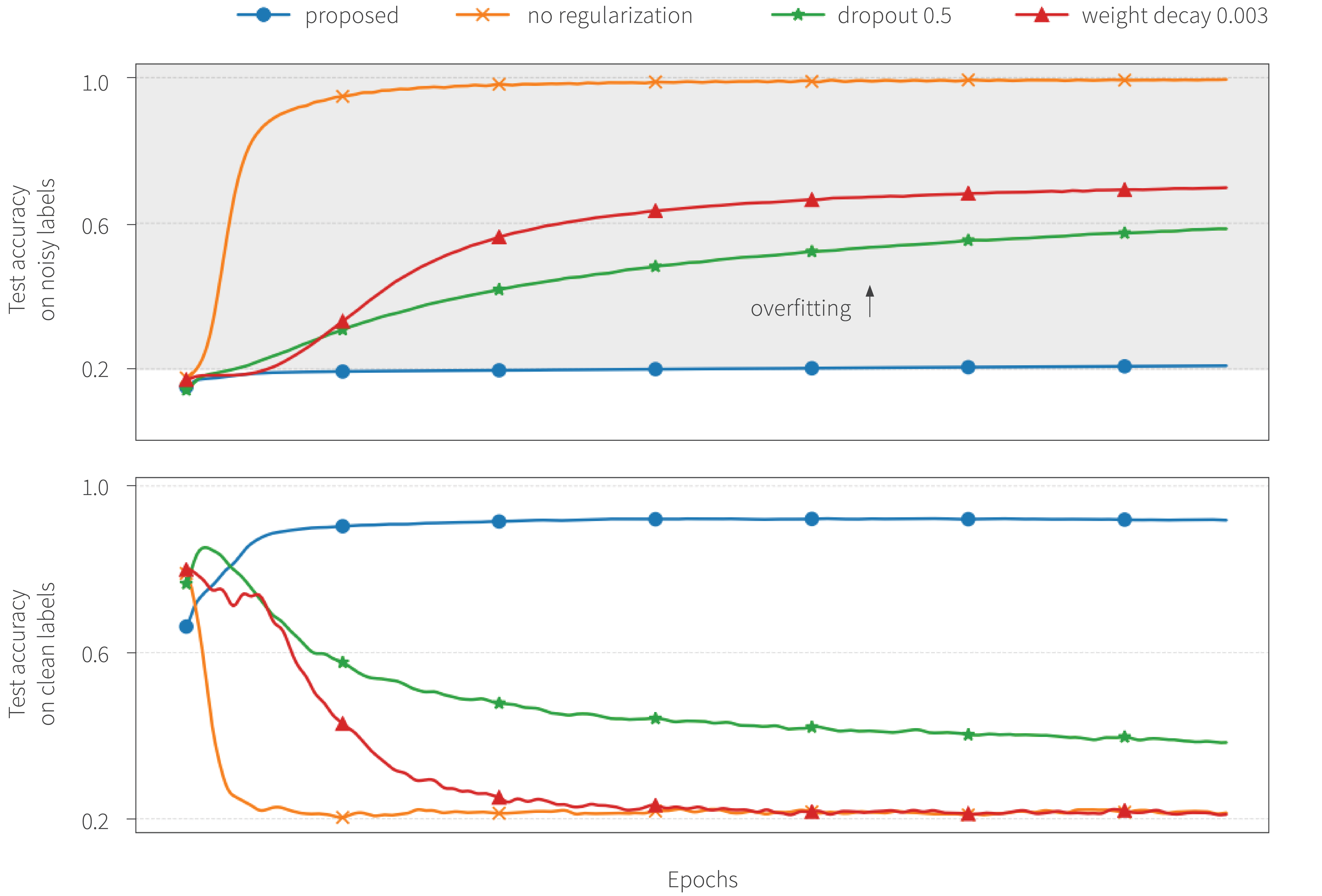
Figure 1. Neural networks tend to memorize labels when trained with noisy labels (80% noise in this case), even when dropout or weight decay are applied. The proposed training approach limits label-noise information in neural network weights, avoiding memorization of labels and improving generalization.
What problem does it solve? Neural networks have the undesirable tendency to memorize information about the noisy labels. This paper shows that, for any algorithm, low values of mutual information between weights and training labels given inputs $I(w : \pmb{y}|\pmb{x})$ correspond to a reduction in memorization of label-noise and better generalization bounds. Novel training algorithms are proposed to optimize for this and achieve impressive empirical performances on noisy data.
Why is this important? Even in the presence of noisy labels, deep neural networks tend to memorize the training labels. This hurts the generalization performance generally and is particularly undesirable with noisy labels. Poor generalization due to label memorization is a significant problem because many large, real-world datasets are imperfectly labeled. From a information-theoretic perspective, this paper reveals the root of the memorization problem and proposes an approach that directly addresses it.
The approach taken and how it relates to previous work: Given a labeled dataset $S=(\pmb{x}, \pmb{y})$ for data $\pmb{x}=\{x^{(i)}\}_{i=1}^n$ and categorical labels $\pmb{y}=\{y^{(i)}\}_{i=1}^n$ and learning weights $w$, Achille & Soatto present a decomposition of the expected cross-entropy $H(\pmb{y}|\pmb{x}, w)$:
\[ H(\pmb{y} | \pmb{x}, w) = \underbrace{H(\pmb{y} | \pmb{x})}_{\text{intrinsic error}} + \underbrace{\mathbb{E}_{\pmb{x}, w}D_{\text{KL}}[p(\pmb{y}|\pmb{x})||f(\pmb{y}|\pmb{x}, w)]}_{\text{how good is the classifier}} – \underbrace{I(w : \pmb{y}|\pmb{x})}_{\text{memorization}}. \]
If the labels contain information beyond what can be inferred from inputs, the model may do well by memorizing the labels through the third term of the above equation. To demonstrate that $I(w:\pmb{y}|\pmb{x})$ is directly linked to memorization, this paper proves that any algorithm with small $I(w:\pmb{y}|\pmb{x})$ overfits less to label-noise in the training set. This theoretical result is also verified empirically, as shown in Figure 1. In addition, the information that weights contain about a training dataset $S$ has previously been linked to generalization (Xu & Raginsky), which can be tightened with small values of $I(w:\pmb{y}|\pmb{x})$.
To limit $I(w:\pmb{y}|\pmb{x})$, this paper first shows that the information in weights can be replaced by information in the gradients, and then introduces a variational bound on the information in gradients. The bound employs an auxiliary network that predicts gradients of the original loss without label information. Two ways of incorporating predicted gradients are explored: (a) using them in a regularization term for gradients of the original loss, and (b) using them to train the classifier.
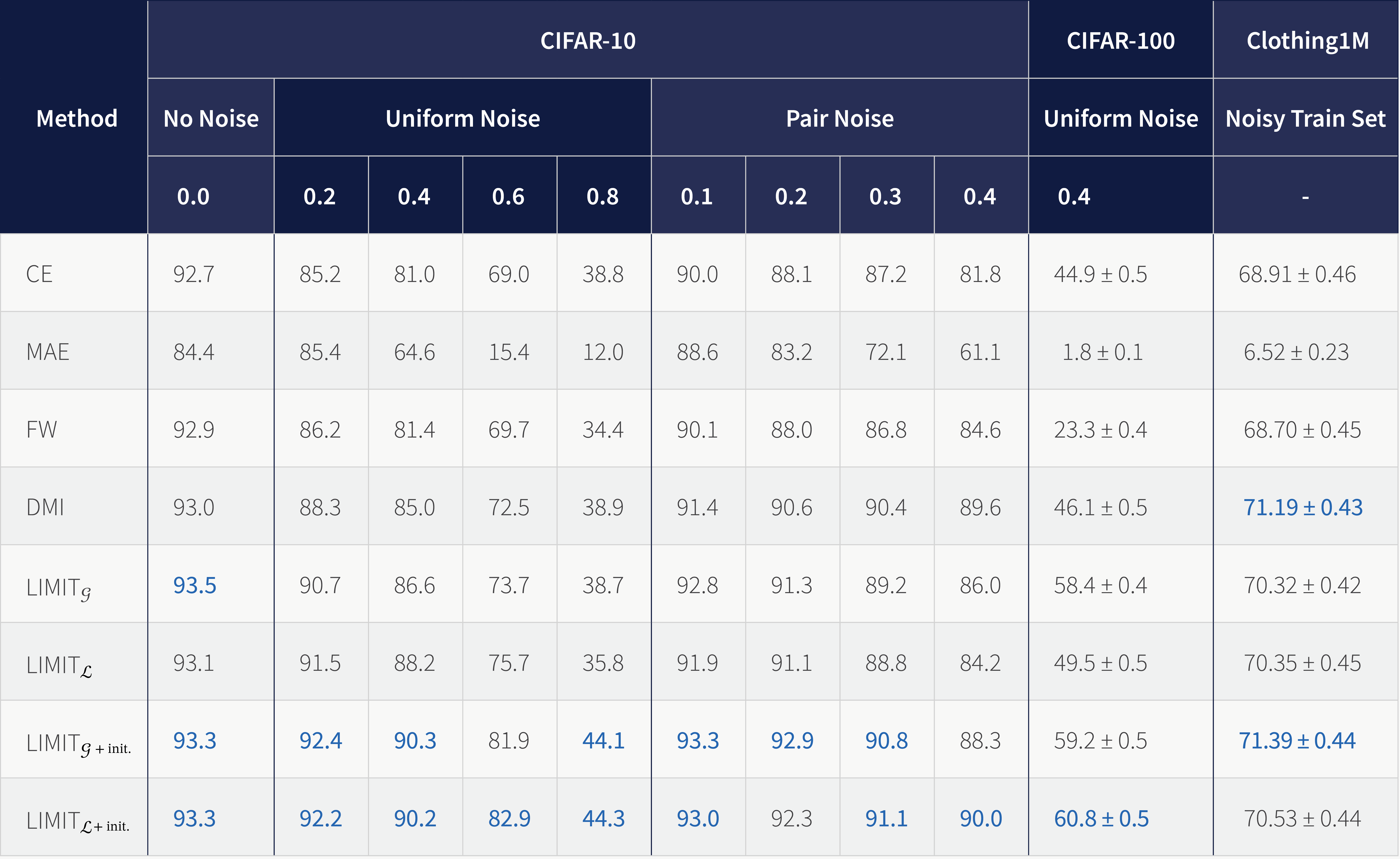
Results: The authors set up experiments with noisy datasets to see how well the proposed methods perform for different types and amounts of label noise. The simplest baselines are standard cross-entropy (CE) and mean absolute error (MAE) loss functions. The next baseline is the forward correction approach (FW) proposed by Patrini et al., where the label-noise transition matrix is estimated and used to correct the loss function. Finally, they include the recently proposed determinant mutual information (DMI) loss proposed by Xu et al., which is the log-determinant of the confusion matrix between predicted and given labels. The proposed algorithm illustrates the effectiveness on versions of MNIST, CIFAR-10 and CIFAR-100 corrupted with various noise models, and on a large-scale dataset Clothing1M that has noisy labels, as shown in Fig 2.

Figure 2. Test accuracy comparison on CIFAR-10, corrupted with various noise types, on CIFAR-100 with 40% uniform label noise and on Clothing1M dataset.
Can Increasing Input Dimensionality Improve Deep Reinforcement Learning?
Kei Ota, Tomoaki Oiki, Devesh K. Jha, Toshisada Mariyama and Daniel Nikovski by Pablo Hernandez-Leal
Related Papers:
What problem does it solve? This paper starts from the question of whether learning good representations for states and using larger networks can help in learning better policies in deep reinforcement learning.
The paper mentions that many dynamical systems can be described succinctly by sufficient statistics which can be used to accurately to predict their future. However, there is still the question whether RL problems with intrinsically low-dimensional state (i.e., with simple sufficient statistics) can benefit by intentionally increasing its dimensionality using a neural network with a good feature representation.
Why is this important? One of the major successes of neural networks in supervised learning is their ability to automatically acquire representations from raw data. However, in reinforcement learning the task is more complicated since policy learning and representation learning happen at the same time. For this reason, deep RL usually requires a large amount of data, potentially millions of samples or more. This limits the applicability of RL algorithms to real-world problems, for example, continuous control and robotics where that amount of data may not be practical to collect.
It can be assumed that increasing the dimensionality of the input might further complicate the learning process of RL agents. This paper argues this is not the case and that agents can learn more efficiently with the high-dimensional representations than with the lower-dimensional state observations. The authors hypothesize that larger networks (with a larger search space) is one of the reasons that allows agents to learn more complex functions of states, ultimately improving sample efficiency.

Figure 3. On the left the diagram of how OFENet outputs, $z_{o_t}$, are the inputs to the RL agent and on the right the standard RL learning process. In both cases the agent learns a policy that outputs an action $a_t$.
The approach taken and how it relates to previous work: The area of state representation learning focuses on representation learning where learned features are in low dimension, evolve through time, and are influenced by actions of an agent. In this context, the authors highlight a previous work by Munk et al. where the output of a neural network is used as input for a deep RL algorithm. The main difference is that the goal of Munk et al. is to learn a compact representation, in contrast to the idea of this paper which is learning good higher-dimensional representations of state observations.
The paper proposes an Online Feature Extractor Network (OFENet) that uses neural networks to produce good representations that are used as inputs to a deep RL algorithm, see Figure 3.
OFENet is trained with the goal of preserving a sufficient statistic via an auxiliary task to predict future observations of the system. Formally, OFENet trains a feature extractor network for the states, $z_{o_t}=\phi_o(o_t)$, a feature extractor for the state-action, $z_{o_t,a_t}=\phi_{o,a}(o_t,a_t)$, and a prediction network $f_{pred}$ parameterized by $\theta_{pred}$. The parameters $\{\theta_o, \theta_{o,a}, \theta_{pred}\}$ are optimized to minimize the loss:
$$L=\mathbb{E}_{(o_t,a_t)\sim p,\pi} [||f_{pred}(z_{o_t},a_t) – o_{t+1}||^2]$$
which is interpreted as minimizing the prediction error of the next state.

Figure 4. OFENet architecture. Observation and action are represented by $o_t$, $a_t$; FC represents a fully connected layer with an activation function, and concat represents a concatenation of the inputs.
The authors highlight the need for a network that can be optimized easily and produce meaningful high-dimensional representations. Their proposal is a variation of DenseNet, a densely connected convolutional network whose output is the concatenation of previous layer’s outputs. OFENet uses a DenseNet architecture and is learned in on online fashion, at the same time as the agents policy, receiving as input observation and action as depicted in Figure 4.
Results: The paper evaluates 60 different architectures with varying connectivity, sizes and activation functions. The results showed that an architecture similar to DenseNet consistently achieved higher scores than the rest.
OFENet was evaluated with both on-policy (SAC and PPO) and off-policy reinforcement learning algorithms (TD3) on continuous control tasks. With these three algorithms the addition of OFENet obtained better results than without it.
Ablation experiments were performed to verify that just increasing the dimensionality of the state representation is not sufficient to improve performance. The key point is that generating effective higher dimensional representations, for example with OFENet, is required to obtain better performance.
Relaxing Bijectivity Constraints with Continuously Indexed Normalising Flows
Rob Cornish, Anthony L. Caterini, George Deligiannidis, and Arnaud Doucet by Ivan Kobyzev
Related Papers:
What problem does it solve? The key ingredient of a Normalizing Flow is a diffeomorphic function (i.e., invertible function which is differentiable and its inverse is also differentiable). To model a complex target distribution a normalizing flow transforms a simple base measure via multiple diffeomorphisms stacked together. However, diffeomorphisms preserve topology; hence, the topologies of the supports of the base distribution and target distribution must be the same. This is problematic for the real-world data distributions which can have complicated topology (e.g., they can be disconnected, have holes, etc). The paper proposes a way to replace a diffeomorphic map with a continuous family of diffeomorphisms to solve this problem.
Why is this important? It is generally believed that many distributions exhibit complex topology. Generative methods which are unable to learn different topologies will, at the very least, be less sample efficient in learning and potentially fail to learn important characteristics of the target distribution.

Figure 5. Generative process for forward generation for Continuously Indexed Flow. Here $U$ is a continuous latent variable which controls the diffeomorphic flow transformation of $Z$ to produce the target distribution $X$.
The approach taken and how it relates to previous work: Given a latent space $\mathcal{Z}$ and a target space $\mathcal{X}$, the paper considers a continuous family of diffeomorphisms $\{ F(\cdot, u): \mathcal{Z} \to \mathcal{X} \}_{u \in \mathcal{U}}$. The generative process of this model is given by
$$z \sim P_Z, \quad u \sim P_{U|Z}(\cdot|Z), \quad x = F(z,u),$$
which is illustrated in Figure 5. There is no closed form expression on the likelihood $p_X(x)$, hence to train the model one needs to use variational inference. This introduces an approximate posterior $q_{U|X} \approx p_{U|X}$, and constructs an variational lower bound on $p_X(x)$ which can be used for training. To increase expressiveness one can then stack several layers of this generative process.
The authors proved that under some conditions on the family $F_u$, the model can well represent a target distribution, even if its topology is irregular. The downside, compared to other normalizing flows, is that model doesn’t allow for exact density computation. However estimates can be computed through the use of importance sampling.
Results: The performance of the method is demonstrated quantitatively and compared against Residual Flows, on which it’s architecture is based. On MNIST and CIFAR-10 in particular it performs better than Residual Flow (Figure 6), improving the bits per dimension on the test set by a small but notable margin. On other standard datasets the improvements are even larger and, in some cases, state-of-the-art.

Figure 6. Test set bits per dimension (lower is better).
How Good is the Bayes Posterior in Deep Neural Networks Really?
Florian Wenzel, Kevin Roth, Bastiaan S. Veeling, Jakub Świątkowski, Linh Tran, Stephan Mandt, Jasper Snoek, Tim Salimans, Rodolphe Jenatton, Sebastian Nowozin by Mohamed Osama Ahmed
Related Papers:
What problem does it solve? The paper studies the performance of Bayesian neural network (BNN) models and why they have not been adopted in industry. BNNs promise better generalization, better uncertainty estimates of predictions, and should enable new deep learning applications such as continual learning. But despite these potentially promising benefits, they remain widely unused in practice. Most recent work in BNNs has focused on better approximations of the posterior. However this paper asks whether the actual posterior itself is the problem, i.e., is it even worth approximating?
Why is this important? If the actual posterior learned by BNN is poor then efforts to construct better approximations are unlikely to produce better results and could actually hurt performance. Instead this would suggest that more efforts should be directed towards fixing the posterior itself before attempting to construct better approximations.
The approach taken and how it relates to previous work: Many recent BNN papers use the “cold posterior” trick. Instead of using the posterior $p(\theta|D) \propto \exp( -U(\theta) )$, where $U(\theta)= -\sum_{i=1}^{n} \log(y_i|x_i,\theta)-\log p(\theta)$, they use $p(\theta|D) \propto \exp(-U(\theta)/T)$ where $T$ is a temperature parameter. If $T=1$, then we recover the original posterior distribution. However, recent papers report good performance with a “cold posterior” where $T<1$. This causes the posterior to become sharper around the modes and the limiting case $T=0$ corresponds to maximum a posteriori (MAP) point estimate.
This paper studies why the cold posterior trick is needed. That is, why is the original posterior learned from BNN is not good enough on its own. The paper investigates three factors:
- Inference: Monte Carlo methods are needed for posterior inference. Could the errors and approximations induced by the Monte Carlo methods cause problems? In particular, the paper studies different problems such as inaccurate SDE simulations, and minibatch noise.
- Likelihood: Since the likelihood function used for training BNNs is the same as the one used for SGD models, then this should not be a problem.
However, the paper raises the point that “Dirty Likelihoods” are used in recent deep learning models. For example batch normalization, dropout, and data augmentation may be causing problems. - Prior: Most BNN work uses a Normal prior over the weights. The paper raises the question of whether this is a good prior which they call the “Bad Prior Hypothesis”. Specifically, the hypothesis is that the current priors used for the parameters of BNNs may be inadequate, unintentionally introducing an incorrect bias into the posterior and potentially being too strong and overruling the data as model complexity increases. To study this the authors draw samples of the BNN parameters $\theta$ from the prior distribution and examine the predictive distribution that results with these randomly generated parameters.
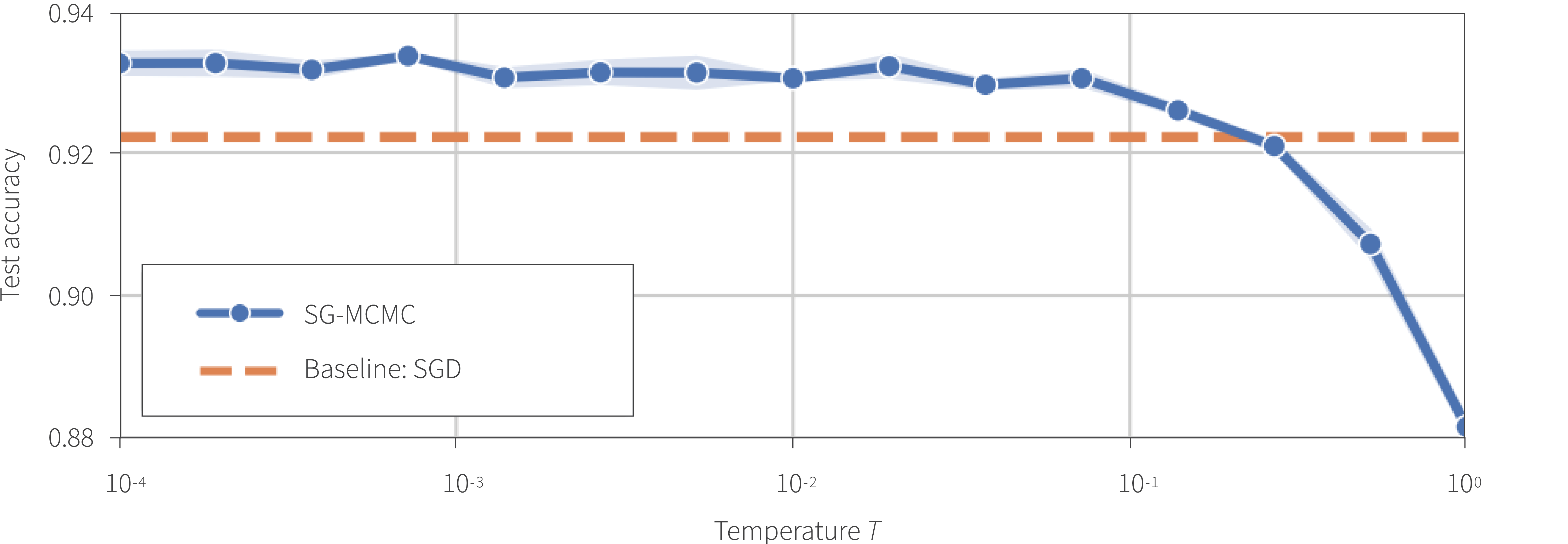
Results: The experiments find that, consistent with previous work, the best posteriors are achieved with cold posteriors, i.e., at temperatures $T<1$. This can be seen in Figure 7. While it’s still not fully understood why, cold posteriors are needed to get good performance with BNNs.
Further, results suggest that neither inference nor the likelihood are the problem. Rather, the prior seems likely to be, at best, unintentionally and misleadingly informative. Indeed, current priors generally map all images to a single class. This is clearly unrealistic and undesirable behaviour of prior. This effect can be seen in Figure 8 which shows the class distribution over the training set for two different samples from the prior.

Figure 7. The “cold posterior;” effect: test accuracy with a ResNet-20 architecture on CIFAR10 with a range of cold ($T<1$) temperatures with the original posterior ($T=1$) on the right. Performance clearly improves with lower temperatures.

Figure 8. The distribution of predicted classes over the training set of CIFAR-10 with two different samples from the prior using a ResNet-20 architecture. In both cases the predicted class distribution is almost exclusively concentrated on a single class which is clearly implausible and undesirable behaviour for the prior.
Discussion
To date there has been a significant amount of work on better approximations for the posterior in BNNs. While this is an important research direction for a number of reasons, this paper suggests that there are other directions that we should be pursuing. This is highlighted clearly by the fact that the performance of BNNs are worse than single point estimates trained by SGD and to improve the performance, cold posteriors are currently required. While this paper hasn’t given a definitive answer to the question of why cold posteriors are needed or why BNNs are not more widely used, it has clearly indicated some important directions for future research.