
This is part II in a series of articles about ordinary differential equations (ODEs) and stochastic differential equations (SDEs) and their application to machine learning. In part I, we introduced ODEs and SDEs and discussed the aspects of machine learning they have been used to describe. In this article, we provide an accessible introduction to ODEs, and in part III we will describe methods to solve first-order ODEs in closed-form. Part V will discuss numerical solutions to ODEs.
In part I we introduced the idea that the ODE is a limit of a discrete sequence as the time interval between updates tends to zero. This article starts by defining ODEs, categorizing types of ODE, and by introducing related terminology. It then discusses what is meant by “solving” an ODE, and describes conditions that determine whether the ODE has a solution. In part III, we’ll see that solutions fall into two categories: closed-form and numerical. We’ll describe the most important techniques for each category.
ODEs
An ordinary differential equation or ODE defines a relation involving the derivatives of a function $\textrm{x}[t]$. For example, we might have:
\begin{equation}
\frac{d^2\textrm{x}[t]}{dt^2} + 0.1 \frac{d \textrm{x}[t]}{dt} = \sin[t] + 1,
\tag{1}
\end{equation}
where $t$ denotes time and $\textrm{x}[t]$ is the function. For the sake of parsimony, we don’t generally write the function explicitly; it would be more typical to write:
\begin{equation}
\frac{d^2 x}{dt^2} + 0.1 \frac{dx}{dt} = \sin[t] + 1.
\tag{2}
\end{equation}
When we talk about solving an ODE, we mean that we find a function $\textrm{x}[t]$ that obeys the constraint that is given by the equation; the ODE can be considered an implicit description of this function.

Figure 1. Example ODE and solutions. This ODE can be represented as a direction field. For each value of $t$ (abcissa) and $x$ (ordinate), the derivative $dx/dt$ is represented as an arrow. If the derivative is zero then the arrow will be horizontal. If it is positive, it will be oriented upwards and if it is negative, it will be oriented downwards. The four lines depict four of the many possible solutions to the equation. Each line follows the arrows in the direction field along its path.
In fact, there is usually a family of functions $\textrm{x}[t]$ that satisfy the equation (figure 1); in the absence of other constraints, the most complete solution to an ODE describes the whole family of functions. Unfortunately, mathematically characterizing the family of solutions for complex ODEs can be difficult. However, for some special classes of ODE, the solutions have a simple relationship. For example, the differential equation:
\begin{equation}
\frac{dx}{dt} = -0.4 \cos[2 t]
\tag{3}
\end{equation}
has solution $x[t]= -0.2 \sin[2 t]+C$ where $C$ is an unknown constant (figure 2). This is easily confirmed by substituting this definition of $x[t]$ into the left-hand side of the original equation and noting that it now equals the right.
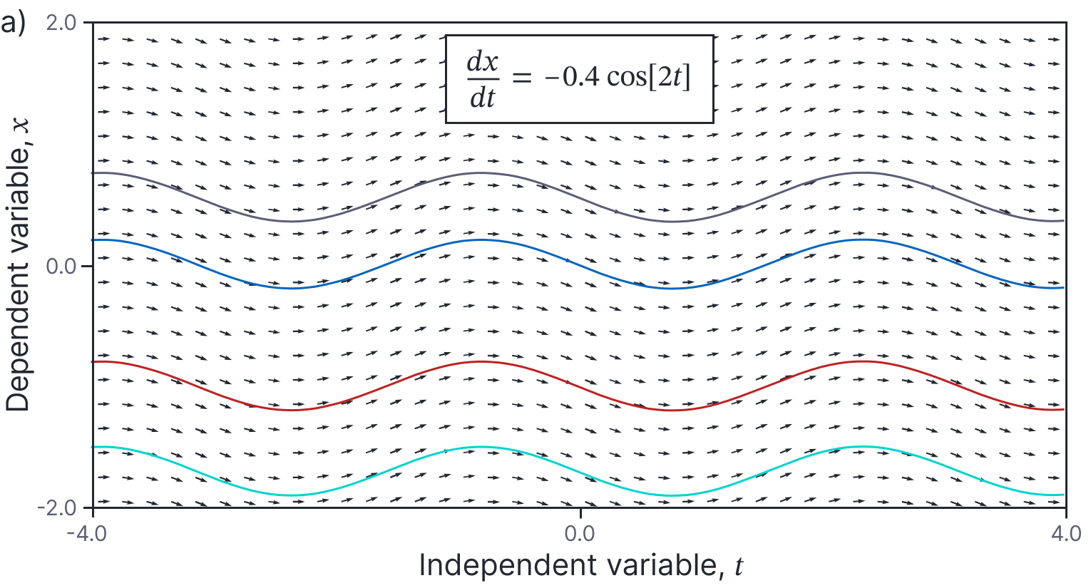
Figure 2. Families of solutions. For some ODEs, the family of solutions can be easily characterized. In this case, each solution is related by an unknown offset, $C$ that has the effect of shifting the solution up or down.
In this example, the member of the family of solutions was determined by the choice of the constant $C$ (representing a vertical offset in figure 2), whereas in figure 1, the solutions have a more complicated relation. One of the goals of this blog is to identify different classes of ODE where the solutions do have simple relations to one another and to characterize those relations. It is these classes for which closed-form solutions are most readily available.
Differential equations in physics
Before we get into the nuts and bolts of ODEs, it’s worth pausing to consider why we would specify a function in this implicit form in the first place. In fact, the study of differential equations originates from the study of physics, where real-world phenomena are commonly described in terms of derivatives. For example, Newton’s second law of motion in one dimension states that:
\begin{equation}
\textrm{f}[t] = m \frac{d^2 x}{dt^2},
\tag{4}
\end{equation}
or in more typical ODE form:
\begin{equation}
\frac{d^2 x}{dt^2} = \frac{1}{m}\cdot \textrm{f}[t],
\tag{5}
\end{equation}
where $x$ is the position of the object, $m$ is its mass, and $\textrm{f}[t]$ is a time-varying force that acts upon the object. If we know the initial position and velocity of the object, we can solve this equation to find its subsequent position as a function of time.
Similarly the one-dimensional heat equation describes how the temperature $T$ varies over time $t$ and position $u$ along a rod of unit length:
\begin{equation}\label{eq:ode2_heat_eqn}
\frac{\partial \textrm{T}[u,t]}{\partial t} = \kappa^2 \frac{\partial^2 \textrm{T}[u,t]}{\partial u^2},
\tag{6}
\end{equation}
where $\kappa^2$ represents the thermal diffusivity of the material. If we know the temperature $\textrm{T}[u, 0]$ at every position $u$ in the rod at time $t=0$ and have some information about what happens at the ends of the rod $\textrm{T}[\bullet, 0]$ and $\textrm{T}[\bullet, 1]$, we can solve this equation to find the temperature $\textrm{T}[u, t]$ at every future time $t$ as a function of the position $u$.
Although ODEs originated in physics, they have since found application in many areas of engineering, including machine learning. These methods are applicable in any situation where we are interested in the cumulative effects of many small local changes.
Terminology and properties of ODE
Unfortunately, the ODE literature is littered with jargon, most of which relates to different categories of equation. This section describes many of these terms.
Terminology
Dependent variable: The function $\textrm{x}[t]$ that we wish to estimate in an ODE is termed the dependent variable.
Independent variable: The quantity $t$ that the dependent variable is a function of is termed the independent variable.
Vector differential equations: In some cases, we have multiple dependent variables $x_{1}, x_{2}\ldots$ and multiple coupled differential equations that relate them. For example, we might have:
\begin{eqnarray}\label{eq:ode2_coupled}
\frac{dx_{1}}{dt} &=& -4 x_{1} + 2 x_{2} + 3\nonumber \\
\frac{dx_{2}}{dt} &=& 3 x_{1} – 5 x_{2} + 2.
\tag{7}
\end{eqnarray}
An ODE with multiple dependent variables $\mathbf{x}\in\mathbb{R}^{D}$ termed a vector differential equation; we can combine the coupled expressions in equation 7 by defining $\mathbf{x}=[x_{1}, x_{2}]^T$ to write a single vector differential equation:
\begin{eqnarray}\label{eq:ode2_vector}
\frac{d\mathbf{x}}{dt} = \begin{bmatrix}-4 & 2 \\ 3 &5 \end{bmatrix}\mathbf{x} +\begin{bmatrix}3\\2\end{bmatrix}.
\tag{8}
\end{eqnarray}
Partial differential equations: Similarly, there is sometimes more than one independent variable. For example, the following equation contains independent variables $u$ and $v$:
\begin{equation}\label{eq:ode2_pde}
x u \frac{\partial^2 x}{\partial u^2} + x^2 uv \frac{\partial^2 x}{dudv} + xv \frac{\partial^2 x}{\partial v^2} +\left(\frac{\partial x}{\partial u}\right)^2 + \left(\frac{\partial x}{\partial v}\right)^2 + x^3 = 0.
\tag{9}
\end{equation}
Since $x[u,v]$ is now a function of more than one quantity, the derivatives become partial derivatives. We refer to this as a partial differential equation or PDE.
Order: The order of a differential equation refers to the highest order derivative that is present in the expression. For example, the example vector ODE in equation 8 is a first-order differential equation and the example PDE in equation 9 is a second-order partial differential equation.
A differential equation of order $n$ with one dependent variable $x$ can be converted to a vector equation in $\mathbf{x}\in\mathbb{R}^n$, by adding extra dependent variables that correspond to each order of derivative. For example, consider the equation:
\begin{equation}
\frac{d^2x}{dt^2} + 2 \frac{d x}{dt} + 3 x = t^2.
\tag{10}
\end{equation}
Now define a new variable $\tilde{x}$ as the first derivative of $x$ so that:
\begin{equation}\label{eq:ode2_new_var_order}
\tilde{x} \triangleq \frac{dx}{dt},
\tag{11}
\end{equation}
and hence:
\begin{equation}
\frac{d\tilde{x}}{dt} = \frac{d^2x}{dt^2}.
\tag{12}
\end{equation}
Then we write:
\begin{eqnarray}
\begin{bmatrix} \frac{dx}{dt} \\ \frac{d\tilde{x}}{dt} \end{bmatrix} &=&
\begin{bmatrix}0 & 1 \\ -3 & -2\end{bmatrix}\begin{bmatrix}x\\\tilde{x}\end{bmatrix} +\begin{bmatrix}0\\t^2\end{bmatrix},
\tag{13}
\end{eqnarray}
where the first line of the equation is just the definition in equation 11, and the second line of the equation is a re-arrangement of the original ODE with only the second derivative term on the left-hand side. We could similarly convert an $n^{th}$ order vector differential equation in $\mathbf{x}\in\mathbb{R}^D$ into a first-order equation in $N\times D$ variables.
Properties of ODEs
This section describe several properties that ODEs may exhibit: time-invariance, linearity, linear homogeneity, and Euler homogeneity. These properties relate to the solubility of the ODE; when one or more of these properties is present, we are more likely to be able to find a closed-form solution.
Time-invariance: Consider an ODE with dependent variable $x$ and an independent variable $t$ that represents time. An ODE is time-invariant if the rate at which $x$ does not depend on the time $t$. For example, these equations are time-invariant:
\begin{eqnarray}
\frac{d^2x}{dt^2} &= & 3\exp[x] \nonumber \\
2\frac{d\mathbf{x}}{dt} – 3 \mathbf{x} & =& 0,
\tag{14}
\end{eqnarray}
whereas these variations are not:
\begin{eqnarray}
\frac{d^2x}{dt^2} &= & 3\exp[x] t^3 \nonumber \\
2\frac{d\mathbf{x}}{dt} – 3 \sin[t]\mathbf{x} & =& \mathbf{A} \mathbf{x} \cdot t.
\tag{15}
\end{eqnarray}
Linearity: An ODE is linear if all terms are proportional to the dependent variable $x$ and its derivatives or are functions of $t$ alone. For example, the following equations are linear:
\begin{eqnarray}
t^2\frac{d^2x}{dt^2} – (t^2+1) x &=& \sin[t] \nonumber \\
\exp[t]\frac{d\mathbf{x}}{dt} – \sin[t]\mathbf{x} &= & \mathbf{0}.
\tag{16}
\end{eqnarray}
Note that the terms in $t$ that multiply $x$ and its derivatives can have any form. The following ODEs are non-linear:
\begin{eqnarray}
\left(\frac{d^2x}{dt^2}\right)^2 – t \frac{dx}{dt} &= & \cos[t]\nonumber \\
t^2\frac{d\mathbf{x}}{dt} – \sin[\mathbf{x}^T\mathbf{x}] \mathbf{x} \cdot t& =& \mathbf{0},
\tag{17}
\end{eqnarray}
because all terms are not proportional to the dependent variable $x$ (or $\mathbf{x}$) or its derivatives; the ODEs include non-linear functions ($\bullet^2, \sin[\bullet^T\bullet]$) of the dependent variables and/or their derivatives. Linearity is important because linear ODEs are easier to solve than non-linear ODEs.
Linear homogeneity: Linear ODEs can be categorized as being homogeneous or inhomogeneous. This is technical distinction, but an important one, since (as we shall see) it is easier to find solutions for homogeneous ODEs. A linear equation is homogeneous if it has the form:
\begin{equation}\label{eq:ode2_linear_homogeneous}
\textrm{a}_{k}[t]\frac{d^kx}{dt^k}+\textrm{a}_{k-1}[t]\frac{d^{k-1}x}{dt^{k-1}} + \ldots + \textrm{a}_{2}[t]\frac{d^2x}{dt^2}+\textrm{a}_{1}[t]\frac{dx}{dt} + \textrm{a}_{0}[t] x =0,
\tag{18}
\end{equation}
where $\textrm{a}_{0}[t]\ldots \textrm{a}_{k}[t]$ are arbitrary functions of $t$. In contrast, a linear equation is inhomogenous if it has the form:
\begin{equation}
\textrm{a}_{k}[t]\frac{d^kx}{dt^k}+\textrm{a}_{k-1}[t]\frac{d^{k-1}x}{dt^{k-1}} + \ldots + \textrm{a}_{2}[t]\frac{d^2x}{dt^2}+\textrm{a}_{1}[t]\frac{dx}{dt} + \textrm{a}_{0}[t] x =\textrm{b}[t].
\tag{19}
\end{equation}
In other words, a linear equation is homogeneous if it has no term $\textrm{b}[t]$ in $t$ alone. In this context the function $\textrm{b}[t]$ is known as a driving term.
Euler Homogeneity: There is a second type of homogeneity that applies to ODEs. A function $\mbox{f}[x, y]$ (not an ODE!) is homogeneous if for any scalar value $\lambda$
\begin{equation}
\mbox{f}[\lambda x,\lambda y] = \lambda^{k} \mbox{f}[x, y],
\tag{20}
\end{equation}
where $k$ is termed the degree. In the context of ODEs, we are usually interested in degree $k=1$, so our working definition of a homogeneous function will be:
\begin{equation}\label{eq:ode2_homog}
\mbox{f}[\lambda x,\lambda y] = \mbox{f}[x, y].
\tag{21}
\end{equation}
If this property holds, then we can rewrite the function $\mbox{f}[x, y]$ as a new function of the ratio of the two inputs $\mbox{h}[x/y]$. This must be true, so that the two factors $\lambda$ on the left-hand side of equation 21 cancel out to yield the right-hand side.
Following from this discussion, we define a first-order differential equation is homogeneous if it has the form:
\begin{equation}
\frac{dx}{dt} = \textrm{h}\left[\frac{x}{t}\right].
\tag{22}
\end{equation}
The following are examples of linear and non-linear Euler homogeneous differential equations, respectively:
\begin{eqnarray}
\frac{dx}{dt} &=&- \frac{x}{t}\nonumber\\
\frac{dx}{dt} &=& -\frac{t(t-x)}{x^2}.
\tag{23}
\end{eqnarray}
For the latter case, you can show that it is homogeneous by re-writing the right-hand side as a function of $x/t$.
Solutions
We now turn to actually solving ODEs. Recall, that this means finding the function or functions $\textrm{x}[t]$ that obeys the ODE.
Families of solutions
ODEs typically have multiple solutions. In other words, there is usually a family of functions $\textrm{x}[t]$ that satisfy the ODE, rather than a single function. For different classes of ODE, the relationship between members of the family will differ. From a mathematical point of view, these families derive from unknown integration constants during the solution process, and so the relationship between members of the family can give us hints about how the equation might be solved. We’ll now consider several different classes of ODEs and see how their solutions are related.
Right-hand side function of $t$ alone: Consider an ODE of the form:
\begin{equation}
\frac{dx}{dt} = \textrm{f}[t]
\tag{24}
\end{equation}
If we are given a solution $\textrm{x}[t]$ that satisfies this equation, then it’s easy to see that $\tilde{\textrm{x}}[t] = C+\textrm{x}[t]$ will also be a solution, where $C$ is an arbitrary scalar constant. This must be true, because the derivatives of $\textrm{x}[t]$ and $\tilde{\textrm{x}}[t]$ with respect to $t$ are the same (figure 3). For similar reasons, some second-order equations have families of solutions related by two unknown constants.
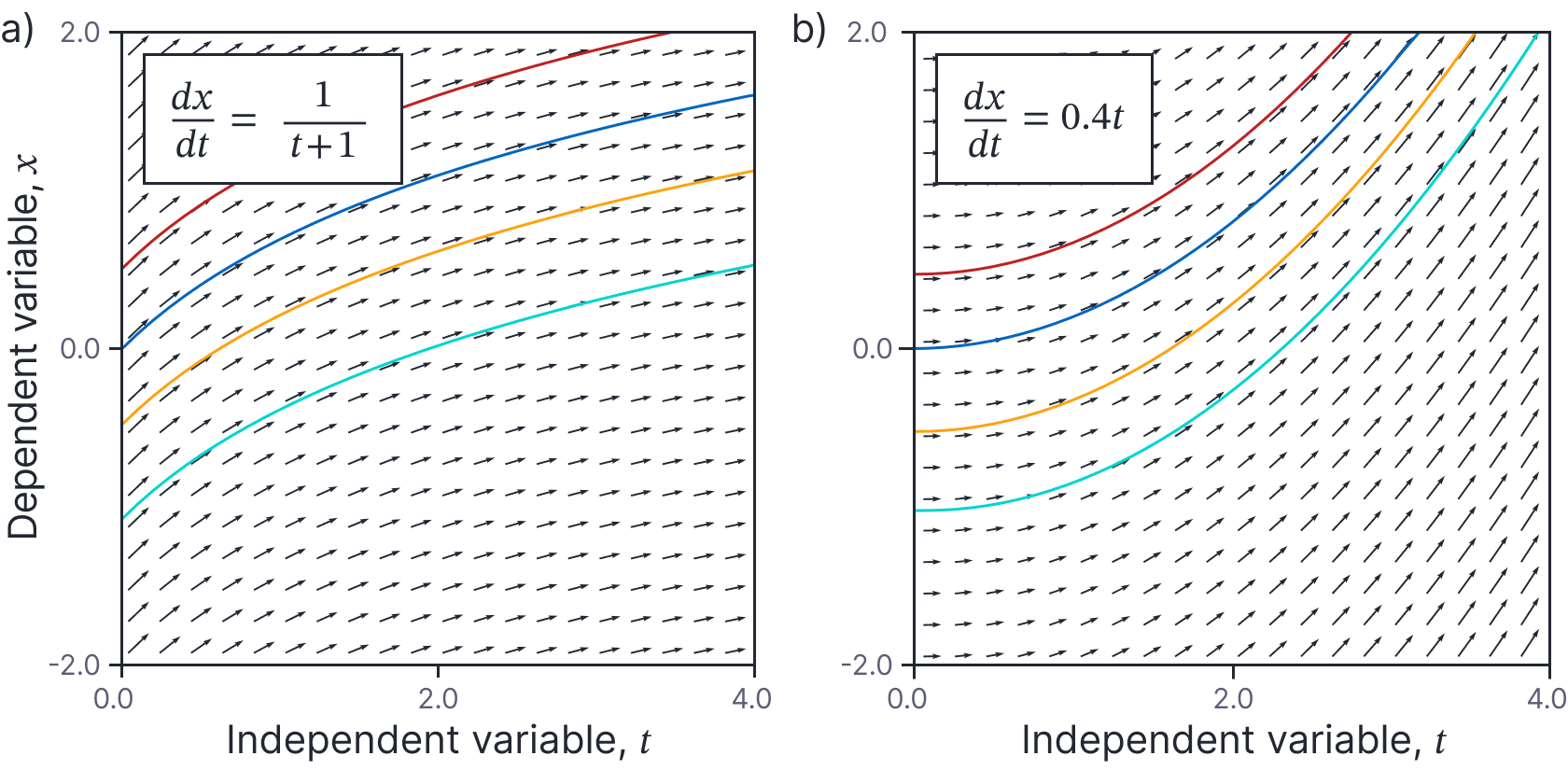
Figure 3. Families of solutions for first-order ODEs when right-hand side is function of $t$ alone. If $\textrm{x}[t]$ is a solution, then so is $\tilde{\textrm{x}}[t] = C+\textrm{x}[t]$, where $C$ is an arbitrary constant. In practice, this means that the solutions are vertically shifted relative to one another on this plot.
Right-hand side function of $x$ alone (time-invariant): Consider a time-invariant ODE of the form:
\begin{equation}
\frac{dx}{dt} = \textrm{f}[x]
\tag{25}
\end{equation}
As you might expect from the name, solutions for time-invariant equations do not depend on the particular time $t$. In other words, time-invariant equations have the property that if $x[t]$ is a solution, then so is $x’=x[t+\tau]$ for any constant $\tau$ (figure 4).
Figure 4. Families of solution for time-invariant ODEs. If $x[t]$ is a solution, then so is $x’=x[t+\tau]$. In practice, this means that the solutions are horizontally shifted relative to one another on this plot.
Linear homogeneous ODEs: Consider any linear, homogeneous ODE such as:
\begin{equation}
\textrm{a}_{2}[t]\frac{d^2x}{dt^2}+\textrm{a}_{1}[t]\frac{dx}{dt} + \textrm{a}_{0}[t] x =0,
\tag{26}
\end{equation}
If we multiply the solution $x[t]$ by some constant $\lambda$, then all the terms in this equation will also be multiplied by $\lambda$:
\begin{equation}
\lambda\cdot \textrm{a}_{2}[t]\frac{d^2x}{dt^2}+\lambda\cdot \textrm{a}_{1}[t]\frac{dx}{dt} + \lambda\cdot \textrm{a}_{0}[t] x =0,
\tag{27}
\end{equation}
Factoring these terms out yields:
\begin{equation}
\lambda\left(\textrm{a}_{2}[t]\frac{d^2x}{dt^2}+\textrm{a}_{1}[t]\frac{dx}{dt} + \textrm{a}_{0}[t] x\right) =0,
\tag{28}
\end{equation}
which must still be true since the term in brackets is equal to zero. It follows that if $x[t]$ is a solution, then $\lambda x[t]$ is also a solution where $\lambda$ is a constant factor (figure 5). Moreover, $x[t]=0$ is always a solution representing the case $\lambda=0$. It’s similarly possible to show that if $x[t]$ is a solution, and $x'[t]$ is a solution of a homogeneous linear ODE, then any combination $\alpha x[t]+\beta x'[t]$ is also a solution.
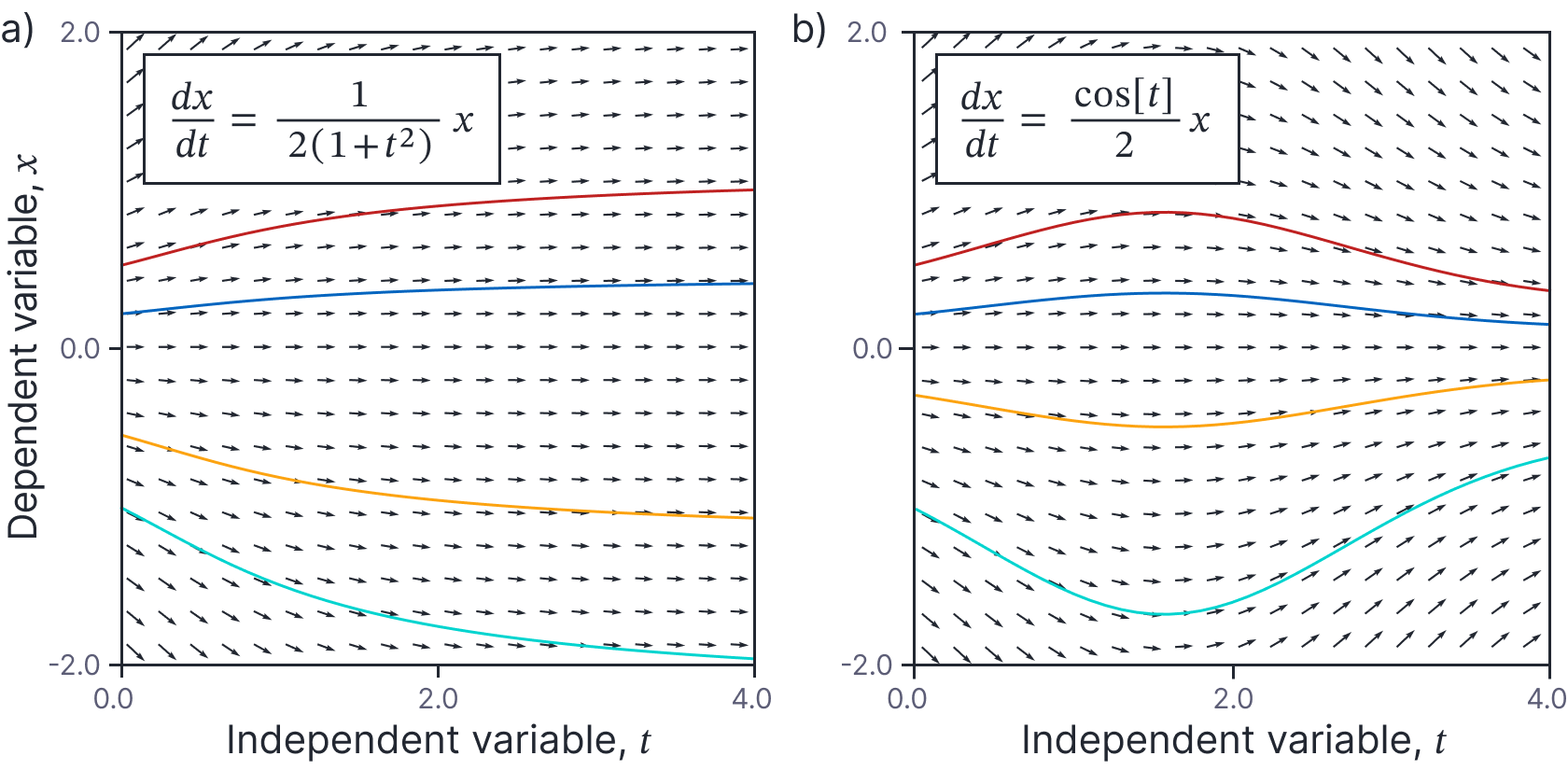
Figure 5. Families of solutions for linear homogeneous first-order ODEs. If $x[t]$ is a solution, then $\lambda x[t]$ is also a solution where $\lambda$ is a constant factor. In practice, this means that the solutions are vertically scaled relative to one another by a constant factor on this plot.
Euler homogeneous ODEs: Consider any Euler homogeneous ODE with the form:
\begin{equation}
\frac{dx}{dt} = \textrm{h}\left[\frac{x}{t}\right].
\tag{29}
\end{equation}
It is straightforward to see that the derivative on the left-hand side of this equation will remain unchanged if we multiply $x$ and $t$ by the same constant $\lambda$. This can be seen in figure 26a-b, where all the arrows along constant ratios of $x/t$ (red dashed lines) have the same orientation. The result of this is that the solutions scale in both $t$ and $x$ as they move further from $t=0, x=0$. This is easily seen in figure 6c where the minimum of the curve occurs at later times $t$ (moves right) the associated value $x$ increases (moves up).
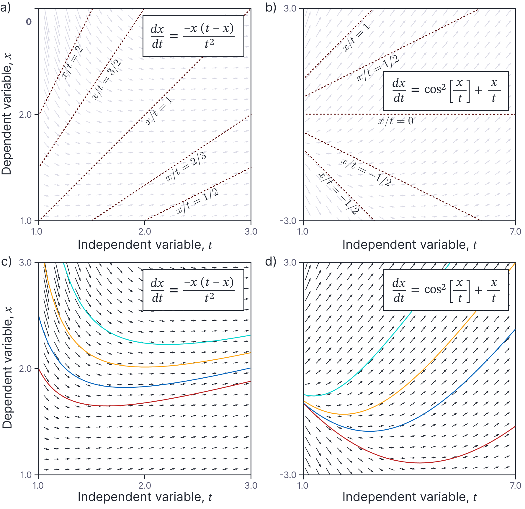
Figure 6. Families of solutions for Euler homogeneous first-order ODEs. a-b) The derivatives for any choice $x/t$ are the same everywhere. In this case, the dashed red lines represent constant values of $x/t$ and the arrows representing the ODE can be seen to identical along each line. c-d) In practice this means that the solutions scale in both $t$ and $x$ according to the distance from $t=0,x=0$.
Boundary conditions
We usually add constraints that determine a particular solution from the larger family of solutions. These constraints are called boundary conditions. There are two types of boundary condition. Initial value boundary conditions (figure 8) specify the value of the independent variable $x$ and possibly its derivatives at some initial value of the dependent variable (usually $t=0$). So, for example, we might have an equation:
\begin{equation}
\frac{d^2x}{dt^2}+ \frac{dx}{dt} = \textrm{f}[t],
\tag{30}
\end{equation}
with initial conditions:
\begin{equation}
x[0] = 2 \quad\quad \textrm{and}\quad\quad \frac{dx[0]}{dt} = -3.
\tag{31}
\end{equation}
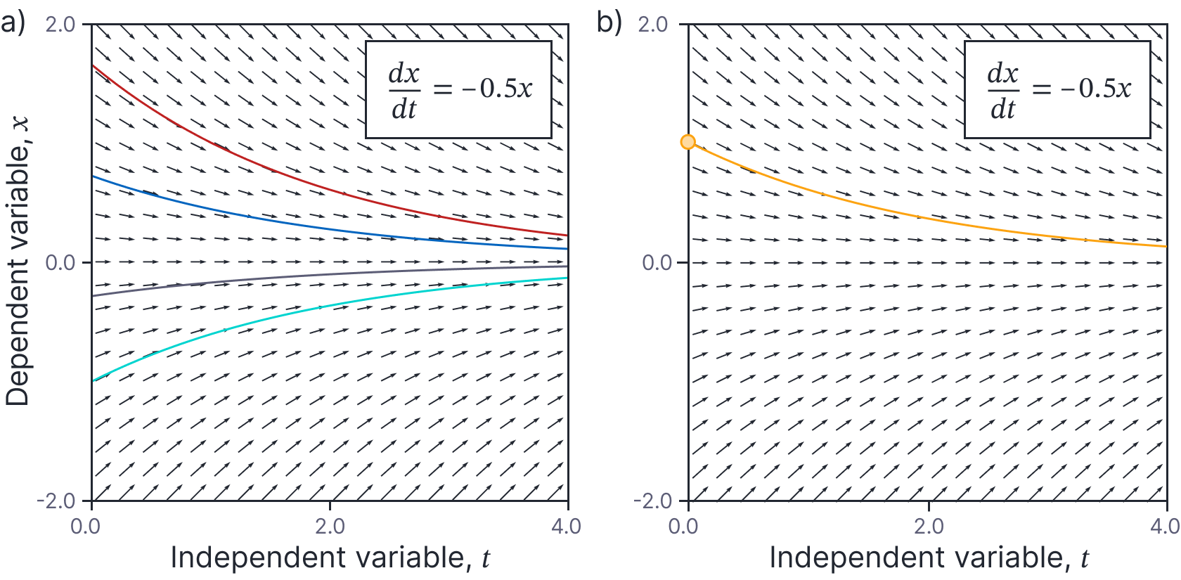
Figure 7. Initial value boundary conditions. a) There is typically a family of solutions to the ODE (four different members of this family shown for this ODE). b) Initial value boundary conditions specify one point on the function, and hence identify one member of this family. In this case, the initial condition $x[0]=1.0$ determines the particular solution.
In contrast boundary value conditions specify the value of the independent variable $x$ at multiple values of the dependent variable. For example, we might specify the boundary values at:
\begin{equation}
x[0] = 2 \quad\quad \textrm{and}\quad\quad x[1] = 0.5.
\tag{32}
\end{equation}
For problems with more than one independent variable, we usually specify constraints that “box in” the solution from several sides. Figure 8 shows one solution of the 1D heat equation (equation 6). It illustrates how the temperature $T[u,t]$ progresses over time, at each position, $u$. Here, we have imposed the initial condition:
\begin{equation}
\mbox{T}[u,0] = 12 \sin\left(\frac{9\pi u}{L}\right)-7 \sin\left(\frac{4\pi u}{L}\right),
\tag{33}
\end{equation}
which specifies the temperature at all positions at time $t=0$ and the boundary value conditions:
\begin{eqnarray}
\mbox{T}[0,t] &=& 0\nonumber \\
\mbox{T}[1,t] &=& 0,
\tag{34}
\end{eqnarray}
which specify the temperature at the ends $u=0,u=1$ of the rod for all times.
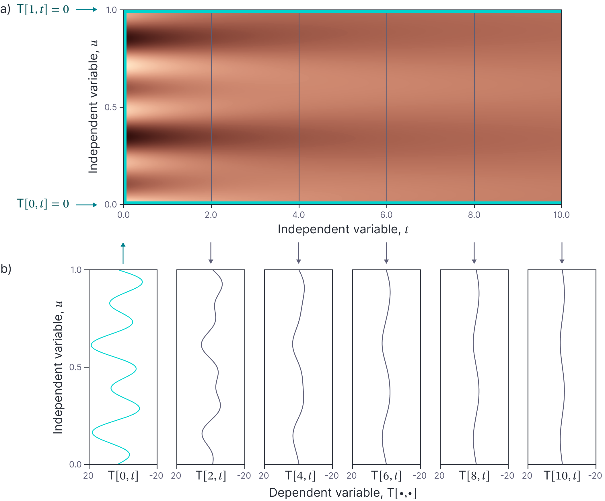
Figure 8. 1D heat equation with boundary conditions. a) This ODE models the change in temperature (dependent variable) in a 1D rod as a function of both the position $u$ and time $t$. Here, the temperature is represented by a the brightness of the color map. Boundary conditions are defined at the three cyan lines. The vertical line represents the initial condition $\textrm{T}[0,t]$ and the two horizontal lines define the boundary value conditions $\textrm{T}[u,0]$ and $\textrm{T}[u,1]$. b) The temperature at times $t=0$ (initial conditions) and subsequently at $t=2,3,6,8,10$.
For both types of boundary condition, we might specify either the value of the solution at certain positions or the derivatives of the solution; in the example above, the boundary value conditions specified the value, but we could alternatively have specified that the derivatives at the boundaries should be zero; this is equivalent to stating that no heat can flow in or out of the bar. When we specify the value of the solution, this is termed a Dirichlet boundary condition. When we specify the derivative, this is termed a Neumann boundary condition.
Existence of solutions
Some combinations of ODEs and boundary conditions don’t have solutions and in other situations, the solution is not unique. It is difficult to know whether a general non-linear ODE has a unique solution. However, for an ODE with the form:
\begin{equation}
\frac{dx}{dt} = \textrm{f}[x,t],
\tag{35}
\end{equation}
and initial condition $x[0], t[0]$, the Picard Lindelof theorem provides two conditions that guarantee that there exists a solution in a range $[t_{0}-\epsilon, t_{0}+\epsilon]$, in a region around $x[0], t[0]$. These conditions are (non-obviously):
- the function $\textrm{f}[x,t]$ is continuous in $t$,
- the function $\textrm{f}[x,t]$ is Lipschitz continuous in $x$ (i.e., is continuous and has derivatives of finite magnitude)
This is sometimes referred to as the fundamental theorem of ordinary differential equations.
Counterexample 1: An ODE that violates the first condition is:
\begin{equation}
\frac{dx}{dt} = \frac{1}{t-1}
\tag{36}
\end{equation}
with boundary condition $x=-1$ at time $t=1$. This has no solution because the right-hand side is not continuous in $t$ at the position specified by the boundary condition (figure 9a).

Figure 9. Existence and uniqueness of solutions. a) This ODE has no solution because right-hand side is not continuous in $t$ (horizontal direction) at the boundary condition (brown circle); the solution tends to negative infinity as it approaches $t-1$ from below and positive infinity from above. b) This ODE has multiple solutions (cyan line is $\textrm{x}[t]= 0$ for all $t$, and brown line is $t^3$ for $t\geq 0$) because the right-hand side is not smooth with respect to $x$ (vertical direction) at the boundary condition (brown circle) and so the function is not Lipschitz continuous. As we move from top to bottom of this plot, the right-hand side decreases until it reaches $x=0$ when it suddenly becomes imaginary (shaded area).
Counterexample 2: An ODE that violates the second condition is:
\begin{equation}
\frac{dx}{dt} = 3 x^{2/3},
\tag{37}
\end{equation}
with boundary condition $x=0$ and $t=0$. This does not violate the first constraint; the right-hand side $\textrm{f}[x,t]$ is constant with respect to $t$. However, right-hand side is not continuous at $x=0$ (it changes suddenly from being real to being imaginary); hence, the derivative of $\textrm{f}[x,t]$ with respect to $x$:
\begin{equation}
\frac{d\textrm{f}[x,t]}{dx} = 2 x^{-1/3} = \frac{2}{\sqrt[3]{x}},
\tag{38}
\end{equation}
is not bounded at $x=0$ and a unique solution is not guaranteed. In fact, there are two possible solutions:
\begin{equation}
\textrm{x}[t] = \begin{cases} 0 & \forall t \\ t^3 & t\geq 0\end{cases}
\tag{39}
\end{equation}
Each of these solutions can be established by substituting the expression for $x$ into the left and right-hand side and establishing that the result is the same. In the first case $\textrm{x}[t]=0$, this is obvious. For the second case, the left and right-hand sides evaluate to:
\begin{eqnarray}
\frac{dx}{dt} &=& \frac{d}{dt}t^3 = 3t^2 \nonumber \\
3x^{2/3} &=& 3 \bigl(t^3\bigr)^{2/3} = 3t^2,
\tag{40}
\end{eqnarray}
respectively (figure 9b).
Note that the related Peano existence theorem places fewer conditions than the Picard Lindelof theorem on the ODE, but makes statements only about the existence of solutions and not their uniqueness.
Conclusion
This blog has introduced ODEs and their associated terminology and discussed what it means to “solve” them. We have seen that ODEs fall into different classes and that the families of the solutions to each class are related in different ways. Finally, we consider the requirements for an ODE to have unique solution. In part III of this series, we’ll show how to solve several prominent classes of ODE in closed form, and describe numerical methods for the other classes for which closed-form solutions are not available.