
In part IX of this series of articles, we saw how stochastic differential equations (SDEs) could be used to describe the evolution of the parameters during the training of neural networks. In part X (this article), we use ordinary differential equations (ODEs) to describe the evolution of the data representation as it passes through a neural network. In the infinitesimal limit, we can consider the neural network as having infinite layers, each of which makes an infinitesimal change to the representation. This is known as a neural ODE.
Neural ODEs have constant memory cost during training and can adapt their evaluation strategy to each input, explicitly trading numerical precision for speed. They can serve as replacements for residual networks but can also be used to perform inference from time-series data that is received at irregular intervals.
We develop neural ODEs by considering what happens when we modify a residual network so that the parameters are shared across all of the layers. We derive an algorithm to compute the gradients for training this network. We then show that inference in this network can be viewed as the Euler numerical method applied to an underlying “neural” ODE. We also find that the calculation of the gradients for training the neural ODE can be viewed as the Euler numerical method applied to a different, but related ODE.
Matrix calculus notation:
Throughout this document, we’ll assume that vectors $\mathbf{x}\in\mathbb{R}^n$ are represented as column vectors and row vectors are denoted by $\mathbf{x}^T$. The Jacobian of a vector function $\textbf{f}:\mathbb{R}^n\rightarrow \mathbb{R}^m$ is an $m\times n$ matrix. It follows that the gradient of a scalar function $\textrm{f}:\mathbb{R}^n\rightarrow \mathbb{R}$, with respect to its $n$-dimensional vector argument is stored in a $1\times n$ row vector.
Residual networks
Residual or skip connections are branches in the computational path of a deep network, whereby the input to each network layer $\textbf{f}[\bullet]$ is added back to the output. For example, a network with four residual blocks is defined as:

Figure 1.1 Residual network with four residual blocks. The input $\mathbf{x}$ is renamed as $\mathbf{z}_0$ and passed through four processing stages to create intermediate representations $\mathbf{z}_1, \mathbf{z}_2, \mathbf{z}_3$, and finally the network output $\mathbf{z}_4$, which is compared to the ground truth output $\mathbf{y}$ using the loss function $\ell[\mathbf{z}_4, \mathbf{y}]$. The $t^{th}$ processing stage consists of applying an additive change $\textbf{f}_{t}[\mathbf{z}_{t-1},\boldsymbol\phi_{t}]$ to the previous representation $\mathbf{z}_{t-1}$.
\begin{align}
\mathbf{z}_{1} &= \mathbf{z}_0 + \textbf{f}_{1}[\mathbf{z}_0,\boldsymbol\phi_{1}]\nonumber \\
\mathbf{z}_{2} &= \mathbf{z}_{1} + \textbf{f}_{2}[\mathbf{z}_{1},\boldsymbol\phi_{2}]\nonumber \\
\mathbf{z}_3 &= \mathbf{z}_{2} + \textbf{f}_{3}[\mathbf{z}_{2},\boldsymbol\phi_{3}]\nonumber \\
\mathbf{z}_4 &= \mathbf{z}_{3} + \textbf{f}_{4}[\mathbf{z}_{3}, \boldsymbol\phi_{4}],
\tag{1.1}
\end{align}
where $\mathbf{z}_0$ is the network input, $\mathbf{z}_4$ is the output, and $\mathbf{z}_{1}$, $\mathbf{z}_{2}$, and $\mathbf{z}_{3}$ denote the intermediate representations (figure 1.1). The functions $\textbf{f}_{t}[\bullet,\boldsymbol\phi_{t}]$ perform the processing and may consist of one or more conventional neural network layers. The first term on the right-hand side of each line is termed the residual connection.
Each function $\textbf{f}_{t}$ learns an additive change to the current representation, and the additive combination of the input and the processed output is known as a residual block or residual layer. Residual connections were originally added to networks to facilitate training with large numbers of layers, which becomes challenging in their absence. Figure 1.2 visualizes the processing of a residual network as a flow field. This hints at a relation with ODEs (which are also often visualized as flow fields).
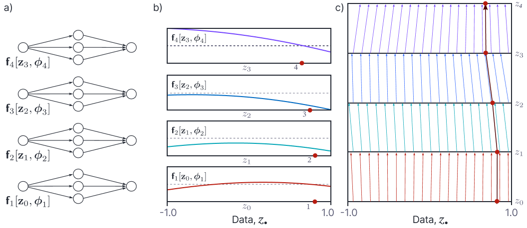
Figure 1.2 Residual network example for scalar input and scalar output. a) The additive function at each layer comprises a neural network with three hidden units and GeLU activations. b) Each of these neural networks defines a function. For a concrete input $z_0$ (red point on $x$-axis of bottom plot), this function returns approximately zero. Consequently, the additive change at block 1 is close to zero and the corresponding input $z_1$ to the second function (red point on $x$-axis of second-to-bottom plot) is approximately the same as $z_0$. The second function returns a negative value for this input and so the additive change is negative and the corresponding input $z_2$ to the next function (red point on third-to-bottom) plot is shifted leftwards. This process continues at each subsequent layer. c) We can visualize the effect of the network by plotting these changes as a flow field. The trajectory of the example point $z_0$ is shown in orange.
Training
Assume that we have training data comprising paired input/output examples $\{\mathbf{x},\mathbf{y}\}$. We set $\mathbf{z}_0=\mathbf{x}$ and run the network to compute $\mathbf{z}_4$. We then define an individual loss function $\ell[\mathbf{z}_4, \mathbf{y}]$ which compares the output $\mathbf{z}_4$ of the network to the output $\mathbf{y}$, and the total loss is the sum of these terms over the whole training set.
To train the network, we use stochastic gradient descent, which requires the derivatives of the individual losses for the data in the current batch with respect to the parameters $\boldsymbol\phi_t$. To make progress, we first calculate the derivatives of the loss with respect to each representation $\mathbf{z}_\bullet$ using the chain rule:
\begin{eqnarray}
&&\mathbf{a}_{4}^T := \frac{d\ell}{d\mathbf{z}_4} \nonumber \\
&&\mathbf{a}_{3}^T := \frac{d\ell}{d\mathbf{z}_3} = \frac{d\ell}{d\mathbf{z}_4}\frac{\partial \mathbf{z}_4}{\partial \mathbf{z}_3} \nonumber \\
&&\mathbf{a}_{2}^T := \frac{d\ell}{d\mathbf{z}_2} = \frac{d\ell}{d\mathbf{z}_4}\frac{\partial \mathbf{z}_4}{\partial \mathbf{z}_3} \frac{\partial \mathbf{z}_3}{\partial \mathbf{z}_2}\nonumber \\
&&\mathbf{a}_{1}^T := \frac{d\ell}{d\mathbf{z}_1} = \frac{d\ell}{d\mathbf{z}_4}\frac{\partial \mathbf{z}_4}{\partial \mathbf{z}_3}\frac{\partial \mathbf{z}_3}{\partial \mathbf{z}_2}\frac{\partial \mathbf{z}_2}{\partial \mathbf{z}_1},
\tag{1.2}
\end{eqnarray}
where we have defined $\mathbf{a}^T_t = d\ell/d\mathbf{z}_t$ (the transpose just identifies this as a row vector). The backbone of the backpropagation algorithm will be the recursion:
\begin{eqnarray}
\mathbf{a}^T_{t} &=& \mathbf{a}^T_{t+1} \frac{\partial \mathbf{z}_{t+1}}{\partial \mathbf{z}_t}\nonumber \\ &=&\mathbf{a}^T_{t+1} + \mathbf{a}^T_{t+1}\frac{\partial \textbf{f}_{t+1}[\mathbf{z}_t, \boldsymbol\phi_{t+1}]}{\partial \mathbf{z}_t},
\tag{1.3}
\end{eqnarray}
where we have substituted the definition of the residual layer $\mathbf{z}_{t+1} = \mathbf{z}_t + \textbf{f}_{t+1}[\mathbf{z}_t,\boldsymbol\phi_{t+1}]$ and taken its derivative with respect to $\mathbf{z}_t$ in the second line.
Finally, we compute the derivative with respect to each set of parameters using:
\begin{eqnarray}
\frac{\partial \ell}{\partial \boldsymbol\phi_t} &=& \frac{\partial \ell }{\partial \mathbf{z}_{t}}\frac{\partial \mathbf{z}_{t}}{\partial \boldsymbol\phi_t}\nonumber\\
&=& \mathbf{a}_t^T \frac{\partial \textbf{f}_t[\mathbf{z}_{t-1}, \boldsymbol\phi_t]}{\partial \boldsymbol\phi_t},
\tag{1.4}
\end{eqnarray}
where we have used the definition of the residual layer $\mathbf{z}_{t} = \mathbf{z}_{t-1} + \textbf{f}_{t}[\mathbf{z}_{t-1},\boldsymbol\phi_{t}]$ and taken its derivative with respect to $\boldsymbol\phi_t$ in the second line. Since the functions $\textbf{f}_t[\mathbf{z}_{t-1}, \boldsymbol\phi_t]$ may themselves contain many neural network layers, there may also be a second inner loop of backpropagation to calculate the terms $\partial \textbf{f}_{t}/\partial \boldsymbol\phi_{t}$.
Residual networks with shared parameters
We’ll gradually modify this residual network to create a neural ODE. As an intermediate step, we first consider using the same function $\textbf{f}[\bullet]$ at each of the four blocks. We parameterize this function by the block index $t$ so that it has a different effect at each step:
\begin{align}
\mathbf{z}_{1} &= \mathbf{z}_{0} + \textbf{f}[\mathbf{z}_0,0, \boldsymbol\phi]\nonumber \\
\mathbf{z}_{2} &= \mathbf{z}_{1} + \textbf{f}[\mathbf{z}_1,1, \boldsymbol\phi]\nonumber\\
\mathbf{z}_3 &= \mathbf{z}_{2} + \textbf{f}[\mathbf{z}_2,2, \boldsymbol\phi]\nonumber \\
\mathbf{z}_4 &= \mathbf{z}_{3} + \textbf{f}[\mathbf{z}_3,3, \boldsymbol\phi].
\tag{1.5}
\end{align}
This model is illustrated in figures 1.3 and 1.4.
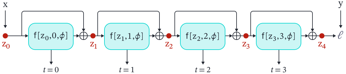
Figure 1.3 Residual network with four residual blocks and shared parameters. The input $\mathbf{x}$ is renamed as $\mathbf{z}_0$ and passed through four processing stages to create intermediate representations $\mathbf{z}_1, \mathbf{z}_2, \mathbf{z}_3$, and finally the network output $\mathbf{z}_4$, which is compared to the ground truth output $\mathbf{y}$ using the loss function $\ell[\mathbf{z}_4, \mathbf{y}]$. The $t^{th}$ processing stage consists of applying an additive change $\textbf{f}[\mathbf{z}_{t-1},t,\boldsymbol\phi]$ to the previous representation $\mathbf{z}_{t-1}$. The parameters are shared between all residual blocks, but the network $\textbf{f}[\mathbf{z}_{t-1},t,\boldsymbol\phi]$ that computes the additive change also takes the block number $t$, so it behaves differently each time.
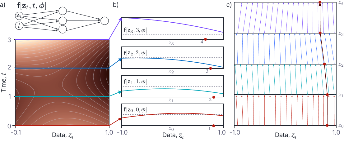
Figure 1.4 Residual network with shared parameters processing for scalar input and scalar output. a) Now the same network $\textbf{f}[\mathbf{z}_{t-1},t,\boldsymbol\phi]$ is shared at each residual block. This has two inputs: the previous data representation $\mathbf{z}_{t-1}$ and the block index (or time) $t$. As such its output can be visualized as a 2D surface. The additive changes at block $t$ for any input $\mathbf{z}$ correspond to the slice through this 2D surface for that value $t$. b) Additive changes at each block as a function of $\mathbf{z}$. c) Additive changes visualized as a flow field.
Training
Let’s now consider how to train this model. To compute the derivative $d\ell/d\boldsymbol\phi$ for the network in equation 1.5, we use the chain rule:
\begin{equation}
\frac{d\ell}{d\boldsymbol\phi} = \frac{d\ell}{d\mathbf{z}_4}\frac{d\mathbf{z}_4}{d\boldsymbol\phi}.
\tag{1.6}
\end{equation}
The first term on the right-hand side is a straightforward derivative that depends on the particular loss function. To compute the second term on the right-hand side, we need to use the total derivative. Consider the situation where we have some function $\textrm{a}\bigl[\theta,\textrm{b}[\theta]\bigr]$ that depends on $\theta$ directly, and also indirectly via the function $\textrm{b}[\theta]$. The total derivative of $\textrm{a}[\bullet,\bullet]$ with respect to $\theta$ is computed as:
\begin{equation}
\frac{da}{d\theta} = \frac{\partial a}{\partial \theta} + \frac{\partial a}{\partial b}\frac{db}{d\theta}.
\tag{1.7}
\end{equation}
Now let’s apply this approach to computing the total derivative $d\mathbf{z}_4/d\boldsymbol\phi$ in equation 1.5 for which $\boldsymbol\phi$ takes the place of $\theta$ and $\mathbf{z}_3[\boldsymbol\phi]$ takes the place of $b[\theta]$:
\begin{equation}
\frac{d\mathbf{z}_4}{d\boldsymbol\phi} = \frac{\partial \mathbf{z}_4}{\partial \boldsymbol\phi} + \frac{\partial \mathbf{z}_4}{\partial \mathbf{z}_3}\frac{d\mathbf{z}_3}{d\boldsymbol\phi}.
\tag{1.8}
\end{equation}
Substituting this result back into equation 1.6, we get:
\begin{equation}
\frac{d\ell}{d\boldsymbol\phi} = \frac{d\ell}{d\mathbf{z}_4}\left(\frac{\partial \mathbf{z}_4}{\partial \boldsymbol\phi} + \frac{\partial \mathbf{z}_4}{\partial \mathbf{z}_3}\frac{d \mathbf{z}_3}{d\boldsymbol\phi}\right).
\tag{1.9}
\end{equation}
We then apply the same approach to the final term $d\mathbf{z}_3/d\boldsymbol\phi$ to yield:
\begin{equation}
\frac{d\ell}{d\boldsymbol\phi} = \frac{d\ell}{d\mathbf{z}_4}\left(\frac{\partial \mathbf{z}_4}{\partial \boldsymbol\phi} + \frac{\partial \mathbf{z}_4}{\partial \mathbf{z}_3}\left( \frac{\partial \mathbf{z}_3}{\partial \boldsymbol\phi} + \frac{\partial \mathbf{z}_3}{\partial \mathbf{z}_2}\frac{d\mathbf{z}_2}{d\boldsymbol\phi}\right)\right),
\tag{1.10}
\end{equation}
and continuing this to its logical end, we get:
\begin{equation}
\frac{d\ell}{d\boldsymbol\phi} = \frac{d\ell}{d\mathbf{z}_4}\left(\frac{\partial \mathbf{z}_4}{\partial \boldsymbol\phi} + \frac{\partial \mathbf{z}_4}{\partial \mathbf{z}_3}\left( \frac{\partial \mathbf{z}_3}{\partial \boldsymbol\phi} + \frac{\partial \mathbf{z}_3}{\partial \mathbf{z}_2}\left( \frac{\partial \mathbf{z}_2}{\partial \boldsymbol\phi} + \frac{\partial \mathbf{z}_2}{\partial \mathbf{z}_1}\left( \frac{\partial \mathbf{z}_1}{\partial \boldsymbol\phi}\right)\right)\right)\right).
\tag{1.11}
\end{equation}
Backpropagation
Equation 1.11 can be used to compute the derivative, but it’s not yet obvious how to reuse elements in a backpropagation style algorithm. We start by multiplying out the terms from equation 1.11:
\begin{equation}
\frac{d\ell}{d\boldsymbol\phi} = \frac{d\ell}{d\mathbf{z}_4} \left(\frac{\partial \mathbf{z}_4}{\partial \boldsymbol\phi} + \frac{\partial \mathbf{z}_4}{\partial \mathbf{z}_3} \frac{\partial \mathbf{z}_3}{\partial \boldsymbol\phi} +\frac{\partial \mathbf{z}_4}{\partial \mathbf{z}_3} \frac{\partial \mathbf{z}_3}{\partial \mathbf{z}_2} \frac{\partial \mathbf{z}_2}{\partial \boldsymbol\phi} +\frac{\partial \mathbf{z}_4}{\partial \mathbf{z}_3} \frac{\partial \mathbf{z}_3}{\partial \mathbf{z}_2} \frac{\partial \mathbf{z}_2}{\partial \mathbf{z}_1} \frac{\partial \mathbf{z}_1}{\partial \boldsymbol\phi}\right).
\tag{1.12}
\end{equation}
This consists of four terms, each starting with $d\ell/d\mathbf{z}_4$, followed by zero or more terms $\partial \mathbf{z}_{t+1}/\partial \mathbf{z}_{t}$ and concluding with a term $\partial \mathbf{z}_t/\partial\boldsymbol\phi$. Denoting:
\begin{align}
&\mathbf{a}_{4}^T := \frac{d\ell}{d\mathbf{z}_4}\nonumber \\
&\mathbf{a}_{3}^T := \frac{d\ell}{d\mathbf{z}_3} = \frac{d\ell}{d\mathbf{z}_4}\frac{\partial \mathbf{z}_4}{\partial \mathbf{z}_3} \nonumber \\
&\mathbf{a}_{2}^T := \frac{d\ell}{d\mathbf{z}_2} = \frac{d\ell}{d\mathbf{z}_4}\frac{\partial \mathbf{z}_4}{\partial \mathbf{z}_3}\frac{\partial \mathbf{z}_3}{\partial \mathbf{z}_2}\nonumber \\
&\mathbf{a}_{1}^T := \frac{d\ell}{d\mathbf{z}_1} = \frac{d\ell}{d\mathbf{z}_4}\frac{\partial \mathbf{z}_4}{\partial \mathbf{z}_3}\frac{\partial \mathbf{z}_3}{\partial \mathbf{z}_2}\frac{\partial \mathbf{z}_2}{\partial \mathbf{z}_1},
\tag{1.13}
\end{align}
we can write:
\begin{align}
\frac{d\ell}{d\boldsymbol\phi} &= \sum_{t=1}^{4}\mathbf{a}^T_{t} \frac{\partial \mathbf{z}_{t}}{\partial \boldsymbol\phi}\nonumber \\
&= \sum_{t=1}^{4}\mathbf{a}^T_{t} \frac{\partial \textbf{f}[\mathbf{z}_{t-1}, t-1, \boldsymbol\phi]}{\partial \boldsymbol\phi},
\tag{1.14}
\end{align}
where we have again used the definition of the residual layer $\mathbf{z}_{t} = \mathbf{z}_{t-1} + \textbf{f}[\mathbf{z}_{t-1}, t-1, \boldsymbol\phi]$ and taken its derivative with respect to $\boldsymbol\phi$ in the second line. We will term this the accumulation equation.
Just as for the original residual network, the backbone of the backpropagation algorithm will be:
\begin{align}
\mathbf{a}^T_{t} &= \mathbf{a}^T_{t+1} \frac{\partial \mathbf{z}_{t+1}}{\partial \mathbf{z}_t}\nonumber \\
&=\mathbf{a}^T_{t+1} + \mathbf{a}^T_{t+1}\frac{\partial \textbf{f}[\mathbf{z}_t, t, \boldsymbol\phi]}{\partial \mathbf{z}_{t}},
\tag{1.15}
\end{align}
where we have substituted the definition of the residual layer $\mathbf{z}_{t+1} = \mathbf{z}_t + \textbf{f}[\mathbf{z}_t, t, \boldsymbol\phi]$ and taken its derivative with respect to $\mathbf{z}_t$ in the second line. We term this the recursion equation.
These are the final backpropagation equations. In the forward pass, we run the residual network (equations 1.15) to compute the values $\mathbf{z}_1, \mathbf{z}_2, \mathbf{z}_{3}, \mathbf{z}_{4}$. Then we start with $\mathbf{a}^T_{4}=\partial \ell/ \partial\mathbf{z}_{4}$ and work backwards, computing the values $\mathbf{a}^T_{3}, \mathbf{a}^T_{2}$ and finally $\mathbf{a}^T_{1}$ using equation 1.15. We accumulate the terms in equation 1.14 as we go.
Neural ODEs
Now we’ll develop the ODE as a shared parameter model with an infinite number of layers. The shared parameter model used residual blocks of the form:
\begin{align}
\mathbf{z}_{t+1} &= \mathbf{z}_t + \textbf{f}[\mathbf{z}_t, t, \boldsymbol\phi],
\tag{1.16}
\end{align}
Note that this equation resembles the Euler integration of an ODE with step size $\Delta t=1$:
\begin{equation}
\mathbf{z}_{t+\Delta t} = \mathbf{z}_{t} + \textbf{f}[\mathbf{z}_t,t, \boldsymbol\phi]\Delta t,
\tag{1.17}
\end{equation}
which we can rearrange to:
\begin{equation}
\frac{\mathbf{z}_{t+\Delta t} – \mathbf{z}_{t}}{\Delta t} = \textbf{f}[\mathbf{z}_t,t, \boldsymbol\phi].
\tag{1.18}
\end{equation}
Since the network is now parameterized by the step $t$, it is perfectly possible to consider using smaller step sizes than $\Delta t = 1$. Taking the limit of both sides as $\Delta t\rightarrow 0$, gives:
\begin{equation}
\frac{d\mathbf{z}}{dt} = \textbf{f}[\mathbf{z},t, \boldsymbol\phi].
\tag{1.19}
\end{equation}
This differential equation describes the evolution of the neural representation as it passes through a network with an infinite number of layers, each of which makes an infinitesimal change. This is known as a neural ordinary differential equation or neural ODE for short (figure 1.5). To compute the output of the network, we solve the differential equation from $t_0$ (the input, usually 0) to $t_1$ (the output, usually 1). This can be done with any numerical ODE solver.
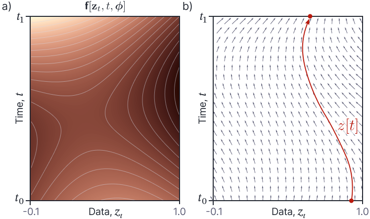
Figure 1.5 Neural ODEs. a) The underlying network is the same as in figure 1.4. b) However, it now defines a continuous flow field over time. Note that where the network gives a smaller output (dark regions in panel a), the flow field acts to decrease the value $z_t$ (arrows in panel b point leftwards). Where it gives a larger output (bright regions in panel a), the flow field acts to increase the value $z_t$ (arrows in panel b point rightwards).
Computing derivatives of loss
The backward pass of the backpropagation algorithm for the shared-parameter model was based on the recursion and accumulation equations:
\begin{equation}
\mathbf{a}_{t}^T = \mathbf{a}_{t+1}^T + \mathbf{a}_{t+1}^T \frac{\partial\textbf{f}[\mathbf{z}_t,t, \boldsymbol\phi]}{\partial \mathbf{z}_{t}},
\tag{1.20}
\end{equation}
and:
\begin{align}
\frac{d\ell}{d\boldsymbol\phi} &= \sum_{t=1}^{4}\mathbf{a}^T_{t} \frac{\partial \textbf{f}[\mathbf{z}_{t-1}, t\!-\!1, \boldsymbol\phi]}{\partial \boldsymbol\phi}.
\tag{1.21}
\end{align}
We can similarly treat the recursion equation as the Euler integration of an ODE with step size $\Delta t=1$ and then take the limit to get the differential equation:
\begin{equation}
\frac{d\mathbf{a}^T}{dt} = -\mathbf{a}^T\frac{\partial\textbf{f}[\mathbf{z}_t,t, \boldsymbol\phi]}{\partial \mathbf{z}_{t}}.
\tag{1.22}
\end{equation}
For reasons that will become clear, we refer to $\mathbf{a}^T$ as the sensitivity in this context and we’ll call this the sensitivity ODE. In the infinitesimal limit, the sum in the accumulation equation becomes an integral to yield:
\begin{equation}
\frac{d\ell}{d\boldsymbol\phi} = \int_{t_0}^{t_1}\mathbf{a}^T\frac{\partial\textbf{f}[\mathbf{z}_t,t, \boldsymbol\phi]}{\partial \boldsymbol\phi} dt.
\tag{1.23}
\end{equation}
We note that this integral can also be viewed as the solution to a third ODE:
\begin{equation}
\frac{d\mathbf{g}}{dt} = \mathbf{a}^T\frac{\partial\textbf{f}[\mathbf{z},t, \boldsymbol\phi]}{\partial \boldsymbol\phi},
\tag{1.24}
\end{equation}
where $\mathbf{g} = d\ell/d\boldsymbol\phi$.
Naive backpropagation algorithm
A naive backpropagation algorithm might hence consist of three stages (figure 1.6):
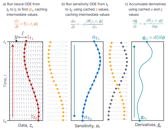
Figure 1.6 Naive backpropagation algorithm. a) We run the neural ODE using the standard Euler numerical method and caching the intermediate values $\mathbf{z}_t$ (orange circles). b) We then run the sensitivity ODE backwards, using the cached $\mathbf{z}_t$ values, and caching the resulting sensitivity values $\mathbf{a}_t$ (gray circles). c) Finally, we run the accumulation ODE forward, using the cached values of both $\mathbf{z}_t$ and $\mathbf{a}_t$. The result at time $t_1$ is the derivative of the loss.
Forward pass: We use a numerical method to solve the network differential equation with the initial value $\mathbf{z}_{t_0}$ being the network input $\mathbf{x}$:
\begin{equation}
\frac{d\mathbf{z}}{dt} = \textbf{f}[\mathbf{z},t, \boldsymbol\phi].
\tag{1.25}
\end{equation}
We store the network representation $\mathbf{z}[k\Delta t]$ for each of the $k$ steps of the numerical algorithm for reuse in the backward pass.
Backward pass: We use the same numerical method to solve the sensitivity ODE backwards in time:
\begin{equation}
\frac{d\mathbf{a}^T}{dt} = -\mathbf{a}^T\frac{\partial\textbf{f}[\mathbf{z},t, \boldsymbol\phi]}{\partial \mathbf{z}},
\tag{1.26}
\end{equation}
with initial value $\mathbf{a}^T_{t_1} = \partial \ell/\partial \mathbf{z}_{t_1}$. Here, we use the cached values of $\mathbf{z}[k\Delta t]$ when computing the second term on the right-hand side. We cache the values $\textbf{a}^T[k\Delta t]$ at each step of the backwards numerical algorithm.
Accumulation: Finally, we accumulate the derivatives from the backward pass by numerically integrating the accumulation equation:
\begin{equation}
\frac{d\mathbf{g}}{dt} = \mathbf{a}^T\frac{\partial\textbf{f}[\mathbf{z},t, \boldsymbol\phi]}{\partial \boldsymbol\phi},
\tag{1.27}
\end{equation}
in which we use both the cached values of $\mathbf{z}[k\Delta t]$ and $\textbf{a}^T[k\Delta t]$. The required derivative $d\ell/d\boldsymbol\phi$ is the final value $\mathbf{g}_{t_1}$.
Efficient backpropagation algorithm
The gradient computation in the previous section has several disadvantages. First, it requires three passes. Second, it requires caching two sets of values and so uses increasing amounts of memory as the step size of the numerical method becomes smaller. Third, we cannot use solvers with adaptive step sizes, because the time steps of the cached values must line up in each pass.
This method can be improved by noting that we can avoid caching the network values $\mathbf{z}[t]$ by running this ODE backwards starting from $\mathbf{z}[t_1]$ in concert with the backward pass. We also note that the integral over $\mathbf{g}$ in the gradient accumulation ODE can be run backwards, and this can also be done simultaneously. These observations lead to the improved method (figure 1.7):
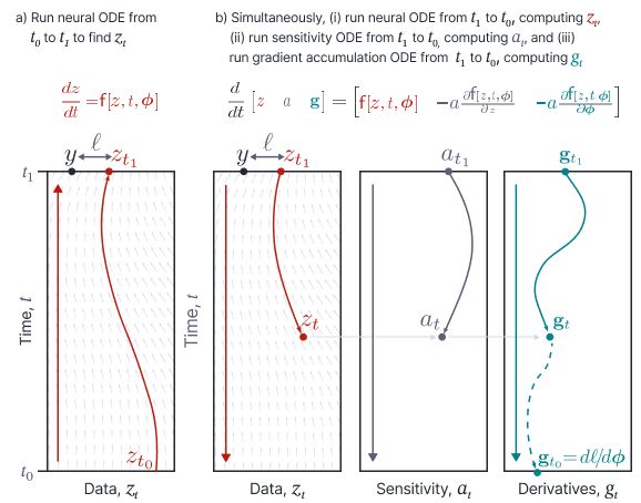
Figure 1.7 Efficient backpropagation algorithm. a) We first run the neural ODE to calculate the output value $z_{t_1}$. b) Then we simultaneously run the neural ODE backwards, run the sensitivity ODE backwards and run the accumulation ODE backwards. At the end, the desired gradient $d\ell/d\boldsymbol\phi$ is the value of the accumulation ODE at time $t_0$.
Forward pass: We solve the network differential equation with the initial value $\mathbf{z}_{t_0}$ being the network input $\mathbf{x}$:
\begin{equation}
\frac{d\mathbf{z}}{dt} = \textbf{f}[\mathbf{z},t, \boldsymbol\phi],
\tag{1.28}
\end{equation}
to yield the network output $\mathbf{z}_{t_1}$.
Backward pass: We concatenate the three output ODEs to form the system:
\begin{equation}
\frac{d}{dt}\begin{bmatrix}
\mathbf{z} &
\mathbf{a}^T &
\mathbf{g}
\end{bmatrix}
= \begin{bmatrix}
\textbf{f}[\mathbf{z},t, \boldsymbol\phi]&
-\mathbf{a}^T\frac{\partial\textbf{f}[\mathbf{z},t, \boldsymbol\phi]}{\partial \mathbf{z}}&
-\mathbf{a}^T\frac{\partial\textbf{f}[\mathbf{z},t, \boldsymbol\phi]}{\partial \boldsymbol\phi}
\end{bmatrix}.
\tag{1.29}
\end{equation}
We solve these combined equations backwards from $t_1$ to $t_0$ with initial conditions:
\begin{equation}
\begin{bmatrix}
\mathbf{z}_{t_1} &
\mathbf{a}^T_{t_1} &
\mathbf{g}_{t_1}
\end{bmatrix}
= \begin{bmatrix}
\mathbf{z}_{t_1} & \frac{\partial \ell}{\partial \mathbf{z}_{t_1}} & \mathbf{0}
\end{bmatrix}.
\tag{1.30}
\end{equation}
When we solve an ODE backwards in time, the change implied by the ODE is multiplied by minus one. This explains the new factor of $-1$ in the last term on the right hand side of equation 1.29; it is required so that when we integrate backwards we still accumulate the derivative correctly. At the end, the desired gradient $d\ell/d\boldsymbol\phi$ is the value $\mathbf{g}_{t_0}$. The minus sign in the ODE for $\mathbf{a}^T$ was intrinsic to its original derivation.
Constrained optimization perspective
We note that the above algorithm is sometimes derived in a completely different way by minimizing the individual loss $\ell[\mathbf{z}_{t_1},\mathbf{y}]$ subject to the constraint that:
\begin{equation}
\frac{d\mathbf{z}}{dt} = \textbf{f}[\mathbf{z}_t, t, \boldsymbol\phi]
\tag{1.31}
\end{equation}
To apply this constraint, we use a continuous form of Lagrange multipliers and form the new loss function $\mathcal{L}[\mathbf{z}_{t_0},\mathbf{y}]$:
\begin{equation}
\mathcal{L}[\mathbf{z}_{t_0},\mathbf{y}] = \ell[\mathbf{z}_{t_1},\mathbf{y}] – \int_{t_0}^{t_1} \boldsymbol\lambda^T \left( \frac{d\mathbf{z}}{dt} – \textbf{f}[\mathbf{z}_t, t, \boldsymbol\phi] \right) dt
\tag{1.32}
\end{equation}
in which the equivalent of the Lagrange multiplier $\boldsymbol\lambda^T[t]$ is now a function of time. In this continuous context, the new loss function $\mathcal{L}[\mathbf{z}_{t_0},\mathbf{y}]$ is called a Lagrangian and the term $\boldsymbol\lambda^T[t]$ is known as the adjoint sensitivity. Applying the calculus of variations to this Lagrangian leads naturally to the same algorithm to compute the gradient, and it turns out that the solution for the adjoint sensitivity $\boldsymbol\lambda^T$ is the term $\mathbf{a}^T[t]$ in our algorithm. This is why we referred to the backward ODE in $\mathbf{a}^T$ as the sensitivity equation. Interested readers can find the derivation in appendix B of this paper.
Stability and reversibility
Gholami et al. (2019) point out two possible numerical problems with the above scheme. They note that this method achieves $\mathcal{O}[1]$ memory complexity because it does not need to cache the intermediate network values during the forward pass. Instead, it recomputes them as it goes by reversing the original ODE. This assumes that the current ODE is numerically stable and can be inverted accurately which is not always the case (figure 1.8).
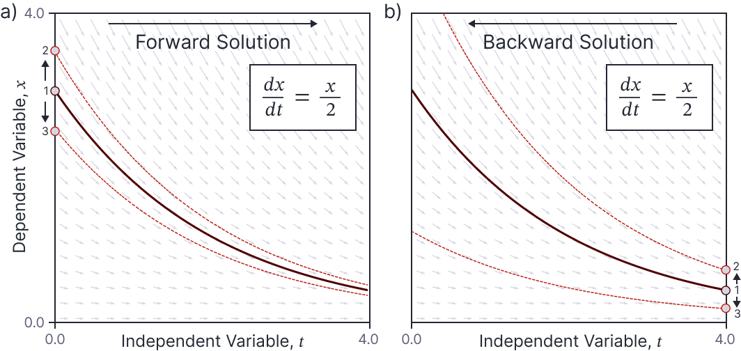
Figure 1.8 Stability of ODEs. a) When we run this ODE forward, a small perturbation to the initial value $x_0$ (from point 1 to points 2 or 3) does not dramatically affect the final outcome. b) However, if we reverse this ODE, a small perturbation to the value $x_{t_1}$ (again from point 1 to points 2 or 3), the solutions diverge widely. We conclude that even if the forward solution of an ODE can be numerically stable, it may still be difficult to run it backwards.
Second, there is a subtle numerical problem in the discretization of this ODE:
\begin{equation}\label{eq:ode10_stability0}
\frac{d\mathbf{a}^T}{dt} = -\mathbf{a}^T\frac{\partial\textbf{f}[\mathbf{z}_t,t, \boldsymbol\phi]}{\partial \mathbf{z}_{t}},
\tag{1.33}
\end{equation}
This was originally defined in the forward direction, where the discrete Euler approximation is:
\begin{equation}
\frac{\mathbf{a}^T_{t+\Delta t}-\mathbf{a}^T_{t}}{\Delta t} = -\mathbf{a}^T_{t}\frac{\partial\textbf{f}[\mathbf{z}_t,t, \boldsymbol\phi]}{\partial \mathbf{z}_{t}},
\tag{1.34}
\end{equation}
which can be rearranged to:
\begin{equation}\label{eq:ode10_stability1}
\mathbf{a}^T_{t} = \mathbf{a}^T_{t+\Delta t}+\mathbf{a}^T_{t}\frac{\partial\textbf{f}[\mathbf{z}_t,t, \boldsymbol\phi]}{\partial \mathbf{z}_{t}}\Delta t.
\tag{1.35}
\end{equation}
However, in practice, we run this in the backwards direction using the backwards Euler method:
\begin{equation}
\frac{\mathbf{a}^T_{t}-\mathbf{a}^T_{t+\Delta t}}{\Delta t} = \mathbf{a}^T_{t}\frac{\partial\textbf{f}[\mathbf{z}_{t+\Delta t},t+\Delta t, \boldsymbol\phi]}{\partial \mathbf{z}_{t+\Delta t}},
\tag{1.36}
\end{equation}
which can be rearranged to:
\begin{equation}\label{eq:ode10_stability2}
\mathbf{a}^T_{t} = \mathbf{a}^T_{t+\Delta t}+\mathbf{a}_{t}^T\frac{\partial\textbf{f}[\mathbf{z}_{t+\Delta t},t+\Delta t, \boldsymbol\phi]}{\partial \mathbf{z}_{t+\Delta t}}\Delta t.
\tag{1.37}
\end{equation}
Notice that the derivatives in equations 1.35 and 1.37 are not the same for finite $\Delta t$; when we run the equations backwards, we are using the network at $t+\Delta t$ not $t$, so in some sense we are replacing the input of the neural network with its output.
The simplest way to handle both of these problems is to return to caching the values of $\mathbf{z}_t$ during the forward pass. Then we do not have to run the original ODE backwards and we can use the appropriate values of $\mathbf{z}_t$ during the backward Euler approximation of equation 1.33. However, this may have very high memory costs.
A compromise is to use a checkpointing approach in which $\mathbf{z}_t$ is cached at a subset of times during the forward pass. The value at any intermediate time can be computed by forward propagating from the nearest cached value. Modern numerical solvers can usually output a value for any specified time so this scheme is compatible with adaptive solvers where we do not know the exact time steps in advance.
Asynchronous time series
The neural ODE above can be substituted directly for a residual network. Here, the network input $\mathbf{x}$ becomes the state $\mathbf{z}_0$ at time $t_0$, and is passed through the ODE to create the output $\mathbf{z}_1$ at time $t_1$. During training we have a single loss $\ell[\mathbf{z}_1, \mathbf{y}]$ that compares the network output to the ground truth target $\mathbf{y}$.
However, neural ODEs can also be used to model asynchronous time-series. For example, consider an unknown physical process that modifies some initial state $\mathbf{x}= \mathbf{z}_0$ over time. For each training example, we are given a set of snapshots $\mathbf{y}_{t_1}, \mathbf{y}_{t_2}, \mathbf{y}_{t_3}\ldots $ of the target over time, where the times $t_1, t_2, t_3\ldots$ may be irregular and different for each training example. For each observation, we have an associated loss function $\ell[\mathbf{z}_{t_{k}}, \mathbf{y}_{t_k}]$ that compares the state of the ODE to the target. A typical choice is the least squares loss function, where the goal is now for the model to replicate the true ODE underlying the physical process as closely as possible.
This situation differs from the original formulation in that each training example $\bigl[\mathbf{x}, \{\mathbf{y}_{t_1}, \mathbf{y}_{t_{2}}, \ldots \mathbf{y}_{t_{K}}\}\bigr] $ has multiple targets and losses associated with different times. A simple way to deal with this would be to split each training example into multiple pairs like $[\mathbf{x},\mathbf{y}_{t_1}]$, $[\mathbf{x}, \mathbf{y}_{t_2}],\ldots [\mathbf{x}, \mathbf{y}_{t_K}]$ and so on. Then we could train the ODE as normal, using a different final time for each example.
A more efficient approach is to incorporate all of the observations into a single forward and backward pass. The forward pass works as normal (figure 1.9a). In the backward pass, we use the simple insight that while the entire trajectory $[0, t_{K}]$ affects the final loss $\ell[\mathbf{z}_{t_{K}} ,\mathbf{y}_{t_K}]$, only the partial trajectory $[0, t_{K-1}]$ affects the penultimate loss $\ell[\mathbf{z}_{t_{K-1}} ,\mathbf{y}_{t_{K-1}}]$, and so on (figure 1.9b). It follows that in the backward pass, we have to gradually incorporate the information from each loss as we reach it while moving backwards in time.
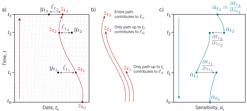
Figure 1.9 Asynchronous time series. a) Forward ODE. The initial point $\mathbf{z}_{t_0}$ is propagated forward in time and its value at times $t_1, t_2$, and $t_3$ are compared to targets $y_{t_1}$, $y_{t_2}$, and $y_{t_3}$, respectively, giving individual losses $\ell_{t_1}$, $\ell_{t_2}$, and $\ell_{t_3}$, respectively. The goal is to change the parameters of the learned ODE (gray arrows) so that the path becomes closer to all of these targets and the sum of these losses decreases. b) We note that only the path up to point $t_1$ contributes to the loss $\ell_{t_1}$, only the path up to point $t_2$ contributes to $\ell_{t_2}$, but the whole path contributes to loss $\ell_{t_3}$. c) The modified backpropagation algorithm initializes the sensitivity equation at time $t_3$ in the normal way to $d\ell_{t_3}/dz_{t_3}$. We then run the sensitivity ODE backwards until time $t_2$ where the loss $\ell_{t_2}$ starts to contribute, at which point, we add $d\ell_{t_2}/dz_{t_2}$ to $a_{t_2}$. We continue backwards until it is time to incorporate $d\ell_{t_1}/dz_{t_1}$, and then finally back to the initial time $t_0$. }
To this end, the final loss is incorporated in the normal way by initializing the adjoint sensitivity to:
\begin{equation}
\mathbf{a}^T = \frac{\partial \ell[\mathbf{z}_{t_{K}}, \mathbf{y}_{t_K}]}{\partial \mathbf{z}_{t_K}}.
\tag{1.38}
\end{equation}
When we reach the position $t_{K-1}$ of the penultimate observation we must incorporate the next loss and we do this by simply adding the derivative $\partial \ell/\partial \mathbf{z}_{t_{K-1}}$ at this point (figure 1.9c):
\begin{equation}
\mathbf{a}_{t_{K-1}}^T\longleftarrow \mathbf{a}_{t_{K-1}}^T+\frac{\partial \ell[\mathbf{z}_{t_{K-1}},\mathbf{y}_{t_{K-1}}]}{\partial \mathbf{z}_{t_{K-1}}}.
\tag{1.39}
\end{equation}
We continue in this way working back through the ODE, incorporating each loss in turn.
Augmented and data-controlled neural ODEs
Consider a 1D mapping from $x$ to $y$ where the output is the negative of the input, so the mapping is $y=-x$. This can easily be represented by a residual network, but not by a neural ODE since the individual paths must overlap to reach their destination (figure 1.10a).
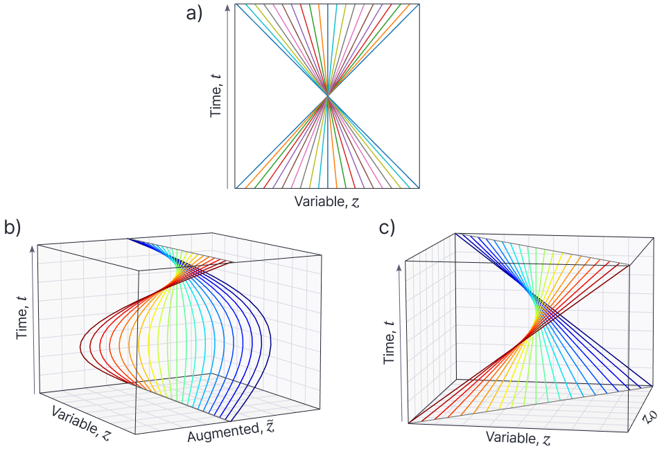
Figure 1.10 Augmented and data-controlled ODEs. a) Consider a mapping from $z_{t_0}$ to $z_{t_1}= -z_{t_0}$. There is no ODE that can represent this because the paths must inevitably overlap somewhere between $z_{t_0}$ and $z_{t_1}$. b) Augmented ODEs add extra dimensions to the data space. This extra dimension allows a mapping from the original variable to its target without the paths overlapping. c) In a data controlled ODE, the neural ODE depends on both the current value $z_{t}$ and the initial value $z_0$. Hence, every initial position is treated differently and once more, a valid mapping from $z_{t_0}$ to $z_{t_1}$ can be achieved.
Augmented neural ODEs tackle this problem by augmenting the data space $\mathbf{z}\leftarrow [\mathbf{z}^T, \tilde{\mathbf{z}}^T]^T$ so that the ODE can use the extra dimensions of $\tilde{\mathbf{z}}$ to compute a valid mapping (figure 1.10b). They replace the original ODE equation and initial conditions:
\begin{equation}
\frac{d\mathbf{z}}{dt} = \textbf{f}[\mathbf{z},t, \boldsymbol\phi], \quad \quad \mathbf{z}_{0} = \mathbf{x}
\tag{1.40}
\end{equation}
with the augmented equation:
\begin{equation}
\frac{d}{dt}\begin{bmatrix}\mathbf{z}\\ \tilde{\mathbf{z}}\end{bmatrix} = \textbf{f}\left[\begin{bmatrix}\mathbf{z}\\ \tilde{\mathbf{z}}\end{bmatrix},t, \boldsymbol\phi\right], \quad \quad \begin{bmatrix}\mathbf{z}_0\\ \tilde{\mathbf{z}}_0\end{bmatrix} = \begin{bmatrix}\mathbf{x}\\ \mathbf{0}\end{bmatrix}.
\tag{1.41}
\end{equation}
Increasing the size of the data representation leads to greater computation per function evaluation which is undesirable. However, experimental evidence suggests that augmented ODEs can model more complex functions using simpler flows and often require fewer function evaluations to solve compared to the original neural ODE.
Data-controlled neural ODEs solve the same problem using a slightly different approach. They pass the original input $\mathbf{x}=\mathbf{z}_{t_0}$ to the network function representing the ODE at every time step, so that each different input is treated differently by the network at the “overlap” points (figure 1.10c):
\begin{equation}
\frac{d\mathbf{z}}{dt} = \textbf{f}\left[\begin{bmatrix}\mathbf{z}\\ \mathbf{z}_0\end{bmatrix},t, \boldsymbol\phi\right], \quad \quad \mathbf{z}_{0} = \mathbf{x}.
\tag{1.42}
\end{equation}
Conclusion
This article has discussed neural ODEs, which represent the evolution of the data representation in a residual network as an ordinary differential equation. Inference is performed by numerically integrating this ODE, and so can exploit all of the features of any modern ODE solver. To learn the neural ODE, we need to compute the derivative of the individual loss function with respect to the parameters. We used the infinitesimal limit of the backward pass of a residual network with shared parameters to show that this gradient can be calculated using two further ODEs. The first sensitivity ODE is equivalent to the backward recursion of the derivative of the loss with respect to the data representation. The second accumulates the effect of the parameters on this representation at each time value.
In the next article, we apply this machinery to make a continuous generative model. In a standard normalizing flow model, a base distribution (usually a normal) is mapped by a series of network layers until it matches the empirical data distribution as closely as possible. In continuous normalizing flows, we consider what happens when we use an ODE to smoothly transform the base distribution to the data distribution.