Neural Tangent Kernel Applications

In part I of this series of blogs, we described gradient flow (gradient descent with infinitesimal steps). We saw that for linear models with least square losses, we can write closed form expressions for the evolution of the residuals, the loss, the parameters, the predictions, and the uncertainty on those predictions.

In part II, we showed that the output of neural networks becomes approximately linear in the parameters when the network width approaches infinity. Hence, we can write similar equations for the training evolution, and these equations depend on the neural tangent kernel or NTK. If there are $I$ training points, the NTK is $I\times I$ where element $(i,j)$ is the dot product between the gradients of the model output with respect to the parameters for training examples $\mathbf{x}_{i}$ and $\mathbf{x}_{j}$. In practice, we can often compute the empirical NTK without explicitly calculating this dot product. We can also compute the expected kernel value in the limit of infinite width. This is known as the analytical NTK.

In this article, we consider the implications of the NTK. We present the expressions for the evolution of the residuals, loss and parameters for neural networks, with a least squares loss and we analyze these expressions to gain insights into trainability and convergence speed. We further write expressions for the evolution of predictions and even their uncertainties over time (neural tangent kernel Gaussian processes). Finally, we show that it is possible to make predictions from an infinitely wide neural network without ever training it explicitly.

*The code related to this blog post can be found on github here.

Trainability and convergence

In part II of this blog, we showed that the evolution of the residuals $\mathbf{f}[\mathbf{X},\boldsymbol\phi]-\mathbf{y}$ is guided by the differential equation:

\begin{eqnarray}\label{eq:NTK3_r_ode}
\frac{d}{dt}\Bigl[\mathbf{f}[\mathbf{X},\boldsymbol\phi]-\mathbf{y}\Bigr] =-\left(\frac{\partial \mathbf{f}[\mathbf{X},\boldsymbol\phi_0]}{\partial \boldsymbol\phi} \frac{\partial \mathbf{f}[\mathbf{X},\boldsymbol\phi_0]}{\partial \boldsymbol\phi}^T\right)\Bigl(\mathbf{f}[\mathbf{X},\boldsymbol\phi]-\mathbf{y}\Bigr),
\tag{1}
\end{eqnarray}

where $\mathbf{X}\in\mathbb{R}^{D\times I}$ contains the $I$ data examples in its columns, $\mathbf{f}[\mathbf{X},\boldsymbol\phi]$ is a model that returns a column vector of length $I$ (i.e., one output for each input) that is compared to targets $\mathbf{y}\in\mathbb{R}^{I}$ using a least squares loss. The bracketed term containing the derivatives is an $I\times I$ matrix and is known as the neural tangent kernel:

\begin{equation}
\mathbf{NTK}\bigl[\mathbf{X},\mathbf{X}\bigr] = \frac{\partial
\mathbf{ f}[\mathbf{X},\boldsymbol\phi_0]}{\partial \boldsymbol\phi} \frac{\partial
\mathbf{ f}[\mathbf{X},\boldsymbol\phi_0]}{\partial \boldsymbol\phi}^T.
\tag{2}
\end{equation}

The ODE in equation 1 can be solved to yield the following relation:

\begin{equation}\label{eq:NTK3_r_ode4}
\mathbf{ f}[\mathbf{X},\boldsymbol\phi_t]-\mathbf{y} = \exp\Bigl[-
\mathbf{ NTK}\bigl[\mathbf{X},\mathbf{X}\bigr]\cdot t\Bigr] \Bigl(
\mathbf{ f}[\mathbf{X},\boldsymbol\phi_0]-\mathbf{y}\Bigr).
\tag{3}
\end{equation}

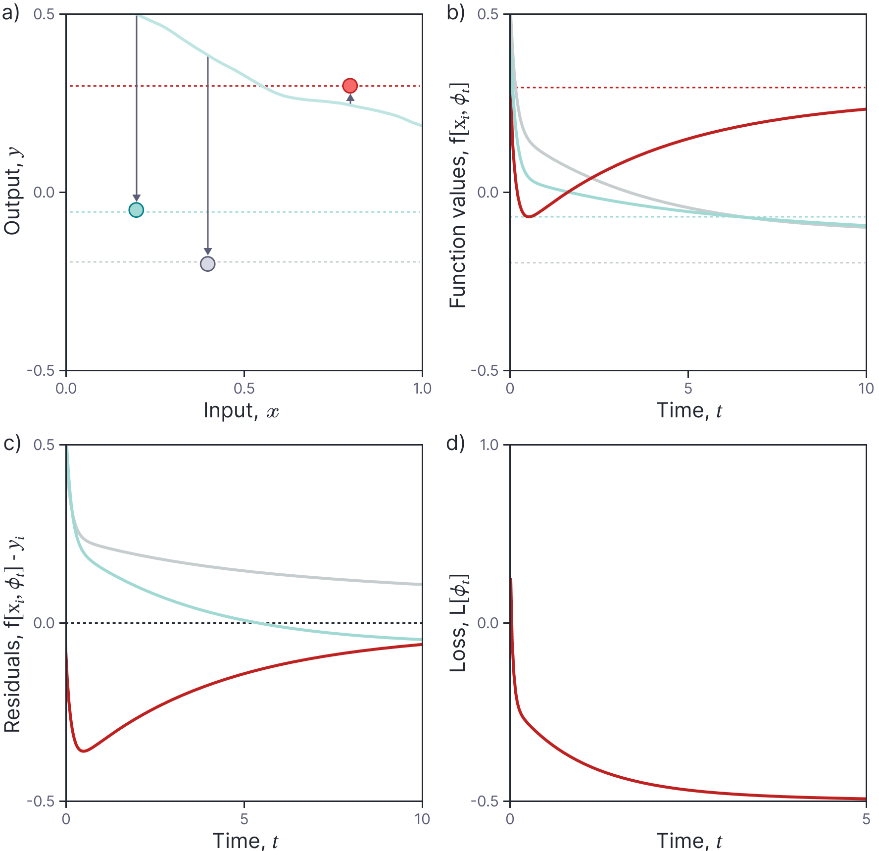
Figure 1 shows the training dynamics for a ReLU network with a single hidden layer containing 15,000 hidden units. The network parameters were initialized from a standard normal distribution, and the neural tangent kernel computed in closed form using the relation:

\begin{eqnarray}\label{eq:NTK3_empirical_kernel_}
\mbox{NTK}[\mathbf{x}_i,\mathbf{x}_{j}] &=& \\
&&\hspace{-1cm}\frac{1}{D}\sum_{d=1}^{D}\omega_{1d}^2 \mathbb{I}\bigl[\boldsymbol\omega_{0d}\mathbf{x}_i > 0\bigr]\mathbb{I}\bigl[\boldsymbol\omega_{0d}\mathbf{x}_j > 0\bigr] \mathbf{x}_i^{T}\mathbf{x}_{j} +\mbox{ReLU}\bigl[\boldsymbol\omega_{0d}\mathbf{x}_{i}\bigr] \mbox{ReLU}\bigl[\boldsymbol\omega_{0d}\mathbf{x}_{j}\bigr]\nonumber,
\tag{4}
\end{eqnarray}

which was derived in part II of this series of blogs.

Figure 1a-b shows the evolution of the function values for the training points. These converge to their targets over time and the residuals decrease to zero (figure 1c). As expected, the loss (the sum of squares of the residuals also decreases to zero (figure 1d).

Trainability and convergence bounds

Equation 3 implies that the residuals will eventually decay to zero as long as the kernel $\mathbf{ NTK}[\mathbf{X},\mathbf{X}]$ is full rank. This will be true as long as no two training inputs $\mathbf{x}_{i}$ and $\mathbf{x}_{j}$ are parallel (see Du et al. 2019), which is usually the case. The change in the loss is bounded above by:

\begin{eqnarray}\label{eq:NTK_eigen_bound}
\frac{dL}{dt} &=& \frac{d}{dt}\biggl[\frac{1}{2}\Bigl(
\mathbf{ f}[\mathbf{X},\boldsymbol\phi] – \mathbf{y}\Bigr)^T\Bigl(
\mathbf{ f}[\mathbf{X},\boldsymbol\phi] – \mathbf{y}\Bigr)\biggr]\nonumber \\ &=& \Bigl(
\mathbf{ f}[\mathbf{X},\boldsymbol\phi_t]-\mathbf{y}\Bigr)^T\frac{d}{dt}\Bigl[
\mathbf{ f}[\mathbf{X},\boldsymbol\phi_t]-\mathbf{y}\Bigr]\nonumber\\
&=& -\Bigl(
\mathbf{ f}[\mathbf{X},\boldsymbol\phi_t]-\mathbf{y}\Bigr)^T
\mathbf{ NTK}\bigl[\mathbf{X},\mathbf{X}\bigr]\Bigl(
\mathbf{ f}[\mathbf{X},\boldsymbol\phi_t]-\mathbf{y}\Bigr)\nonumber \\
&\leq& -\lambda_{I}\Bigl\lVert
\mathbf{ f}[\mathbf{X},\boldsymbol\phi_t]-\mathbf{y} \Bigr\rVert^2,\nonumber\\
&=& -2\lambda_{I}L[\boldsymbol\phi_t],
\tag{5}
\end{eqnarray}

where the third line follows from equation 1 and $\lambda_{I}$ is the smallest eigenvalue of $\mathbf{ NTK}[\mathbf{X},\mathbf{X}]$. This implies (via Grönwall’s inequality) that the loss itself is bounded above by:

\begin{equation}\label{eq:NTK:du_bound}
L[\boldsymbol\phi_{t}] \geq \exp\bigl[-2 \lambda_I t\bigr] L[\boldsymbol\phi_{0}].
\tag{6}
\end{equation}

This shows that the smallest eigenvector of the NTK determines the slowest possible training speed. The ratio between the largest and smallest eigenvalues is sometimes used as a measure of trainability.

This is a remarkable result as it explains why neural networks (at least with infinite widths) are reliably trainable despite the fact that we might initially have expected the loss function to be non-convex and with multiple local minima.

Trainability and labels

The bound in equation 6 is valid, but it doesn’t depend on the targets $\mathbf{y}$. However, we know from experimental evidence that deep networks train more slowly when the targets are randomized. Arora et al. (2019) proposed another bound that takes account of the targets.

We start again with the equation for the evolution of the residual:

\begin{equation}\label{eq:NTK_r_ode4}
\mathbf{ f}[\mathbf{X},\boldsymbol\phi_t]-\mathbf{y} = \exp\Bigl[-
\mathbf{ NTK}\bigl[\mathbf{X},\mathbf{X}\bigr]\cdot t\Bigr] \Bigl(
\mathbf{ f}[\mathbf{X},\boldsymbol\phi_0]-\mathbf{y}\Bigr).
\tag{7}
\end{equation}

Now consider what happens if we arrange the initial output of the network to be zero for every training example. We could do this by subtracting the output of a copy of the network with the same initial parameters from the main network’s output. This leaves the update equation:

\begin{equation}\label{eq:NTK_r_ode_arora}
\mathbf{ f}[\mathbf{X},\boldsymbol\phi_t]-\mathbf{y} = -\exp\Bigl[-
\mathbf{ NTK}\bigl[\mathbf{X},\mathbf{X}\bigr]\cdot t\Bigr] \mathbf{y}.
\tag{8}
\end{equation}

We can express the targets $\mathbf{y}$ in the basis of the the eigenvectors $\mathbf{v}_{1}\ldots \mathbf{v}_{I}$ of the kernel matrix $
\mathbf{ NTK}[\mathbf{X},\mathbf{X}]$ so that $\mathbf{y} = \sum_{i}(\mathbf{v}_{i}^{T}\mathbf{y})\mathbf{v}_{i}$. Then, following equation 5, we have:

\begin{eqnarray}
L[\boldsymbol\phi_{t}] = \frac{1}{2}\Big\lVert
\mathbf{ f}[\mathbf{X},\boldsymbol\phi_t]-\mathbf{y}\Big\rVert^2 &=& \frac{1}{2}\mathbf{y}^T\exp\Bigl[-2
\mathbf{ NTK}\bigl[\mathbf{X},\mathbf{X}\bigr]\cdot t\Bigr] \mathbf{y}\nonumber \\
&=& \frac{1}{2}\sum_{i=1}^{I} \exp\bigl[-2\lambda_i t\bigr](\mathbf{v}_{i}^T\mathbf{y})^2\nonumber\\
&\geq& \frac{1}{2}\min_{i}\Bigl[ \exp\bigl[-2\lambda_i t\bigr](\mathbf{v}_{i}^T\mathbf{y})^2\Bigr]
\tag{9}
\end{eqnarray}

Now we can see that the loss is bounded above by a factor that depends on eigenvalue $\lambda_i$ times the projection of the labels $\mathbf{y}$ onto the corresponding eigenvector.

Figure 2 shows how the decrease in the loss is slower when the labels are randomized on the CIFAR database. This can be explained by the fact that the eigenspectrum of random labels is roughly flat and so has significant energy in directions where the NTK has small eigenvalues, and hence training is slow.

Bounds for finite width networks

The bounds in the previous section are for networks of infinite width, so the neural tangent kernel is constant. To make these practical, we need to prove that when the width is sufficient, the gradient descent path does not diverge by too much from that in the infinite limit. In practice, this means showing that the empirical neural tangent kernel is not too different from that for the analytic (infinite width) case, and that it does not change too much during the optimization process. For more information about these types of proof, consult this blog.

Using these ideas, Du et al. 2019 considered the case where we initialize the weights of a shallow network according to a standard normal distribution and run (discrete) gradient descent with learning rate $\alpha$. They showed that if the width of the network is $\Omega[I^6/(\lambda_0^4\delta^3)]$ and the learning rate $\alpha=\mathcal{O}[\lambda_{0}/I^2]$ then with probability $\delta$:

\begin{eqnarray}
L[\boldsymbol\phi_{t+1}] &\leq& \left(1-\frac{\alpha\lambda_0}{2}\right) L[\boldsymbol\phi_{t}],
\tag{10}
\end{eqnarray}

and the network converges. This is essentially a discrete time version of the first of the bounds derived above.

Similarly, Arora et al. (2019) considered shallow neural networks where the parameters are initialized with variance $\sigma^2_{\boldsymbol\phi} = \mathcal{O}[\epsilon\delta/\sqrt{I}]$. They show that when the width of the network is $\Omega[I^6/(\lambda_0^4,\sigma^4_{\boldsymbol\phi},\delta^4,\epsilon^2)$ and the learning rate is $\alpha=\mathcal{O}[\lambda_{0}/I^2]$ then:

\begin{eqnarray}
\Bigl\lVert
\mathbf{ f}[\mathbf{X},\boldsymbol\phi_t]-\mathbf{y}\Bigr\rVert_2 = \sqrt{\sum_{i=1}^{I}(1-\alpha\lambda_{i})^{2t}(\mathbf{v}_{i}^{T}\mathbf{y})^2}\pm\epsilon,
\tag{11}
\end{eqnarray}

where $\mathbf{v}_i$ is the eigenvector corresponding to the $i^{th}$ eigenvalue of $\mbox{NTK}[\mathbf{X},\mathbf{X}]$. This corresponds to a discretized version of the second of the bounds derived above.

These bounds provide insight into why neural networks are easy to train in practice. Although it is reassuring to know that these bounds exist, it should be emphasized that they are not tight enough to explain empirical performance. Although networks are generally overparameterized, the width of the network does not typically increase with the number of samples $I$ raised to the power of six. However, this work is a start towards understanding why training converges reliably in overparameterized networks.

Evolution of parameters

In equation 16 of part I of this series of blogs, we derived an expression for the evolution of the parameters of a linear model under gradient flow. The equivalent expression for a neural network is given by:

\begin{eqnarray}\label{eq:ntk_four_parameter_evo_general}
\boldsymbol\phi_t&=&\boldsymbol\phi_0 – \frac{\partial
\mathbf{ f}[\mathbf{X},\boldsymbol\phi_0]}{\partial \boldsymbol\phi}^+ \biggl(\mathbf{I}-\exp\Bigl[-
\mathbf{ NTK}\bigl[\mathbf{X},\mathbf{X}\bigr]\cdot t\Bigr]\biggr) \Bigl(
\mathbf{ f}[\mathbf{X},\boldsymbol\phi_0]-\mathbf{y}\Bigr),\nonumber
\tag{12}
\end{eqnarray}

where $\mathbf{A}^+$ denotes the Moore-Penrose inverse of $\mathbf{A}$. In this case, the system will be overdetermined (there are more parameters than training points when the network width is large), and so this is given by $\mathbf{A}^+=\mathbf{A}(\mathbf{A}^{T}\mathbf{A})^{-1}$. This yields:

\begin{eqnarray}\label{eq:ntk3_four_parameter_evo_general2}
\boldsymbol\phi_t\!&\!=\!&\!\boldsymbol\phi_0 – \frac{\partial
\mathbf{ f}[\mathbf{X},\boldsymbol\phi_0]}{\partial \boldsymbol\phi}
\mathbf{ NTK}\bigl[\mathbf{X},\mathbf{X}\bigr]^{-1}\biggl(\mathbf{I}-\exp\Bigl[-
\mathbf{ NTK}\bigl[\mathbf{X},\mathbf{X}\bigr]\cdot t\Bigr]\biggr) \Bigl(
\mathbf{ f}[\mathbf{X},\boldsymbol\phi_0]-\mathbf{y}\Bigr),\nonumber
\tag{13}
\end{eqnarray}

where we have used the fact that the neural tangent kernel $\mathbf{ NTK}[\mathbf{X},\mathbf{X}]$ is the inner product of the derivatives at the initial parameters.

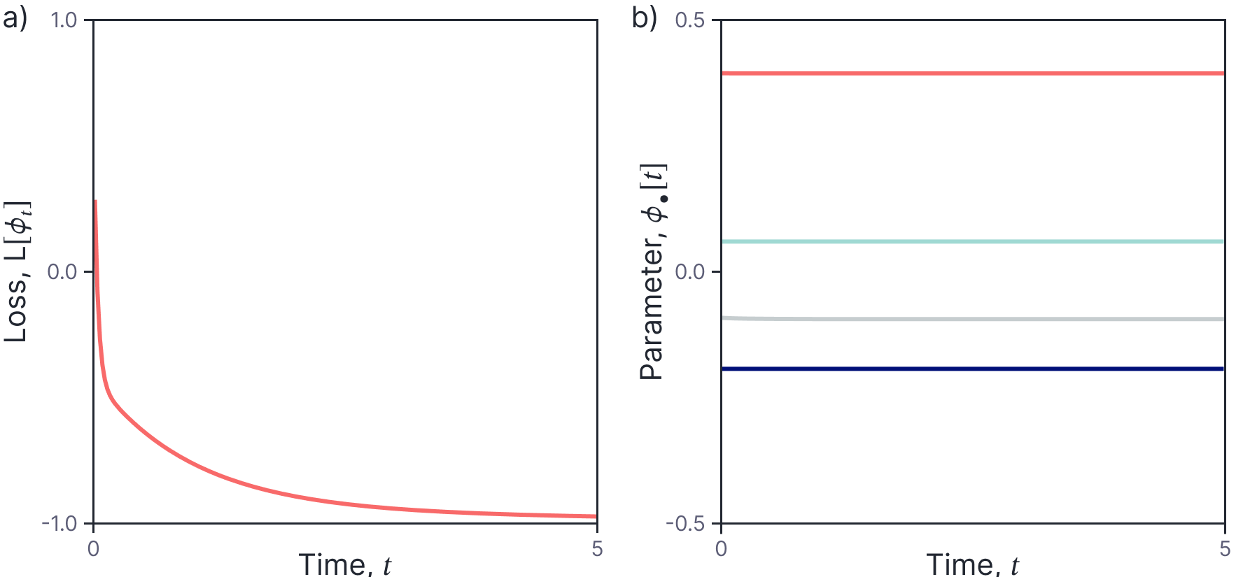
Figure 3 continues the example from figure 1. Although the loss decreases quickly as a function of time, the parameters are almost constant. This shallow network has 15,000 hidden units so there are 15,000 weights and 15,000 biases connecting the input to the single hidden layer and 15,000 weights and 1 bias connecting the hidden layer to the output. The responsibility for changing the model predictions is divided between the 45,001 parameters so any individual parameter changes a very small amount. This is in accordance with other empirical observations (see figure 1 of part II of this series).

Evolution of predictions

Since, we have a closed form expression for the evolution of the network parameters, we evaluate the model using these parameters and visualize the prediction of the model $y^*$ over time for a new data point $\mathbf{x}^{*}$:

\begin{equation}\label{eq:NTK3_pred_evo_full}
y^*_{t} = \mbox{f}\Bigl[\mathbf{x}^{*}, \boldsymbol\phi_{t}\Bigr]
\tag{14}
\end{equation}

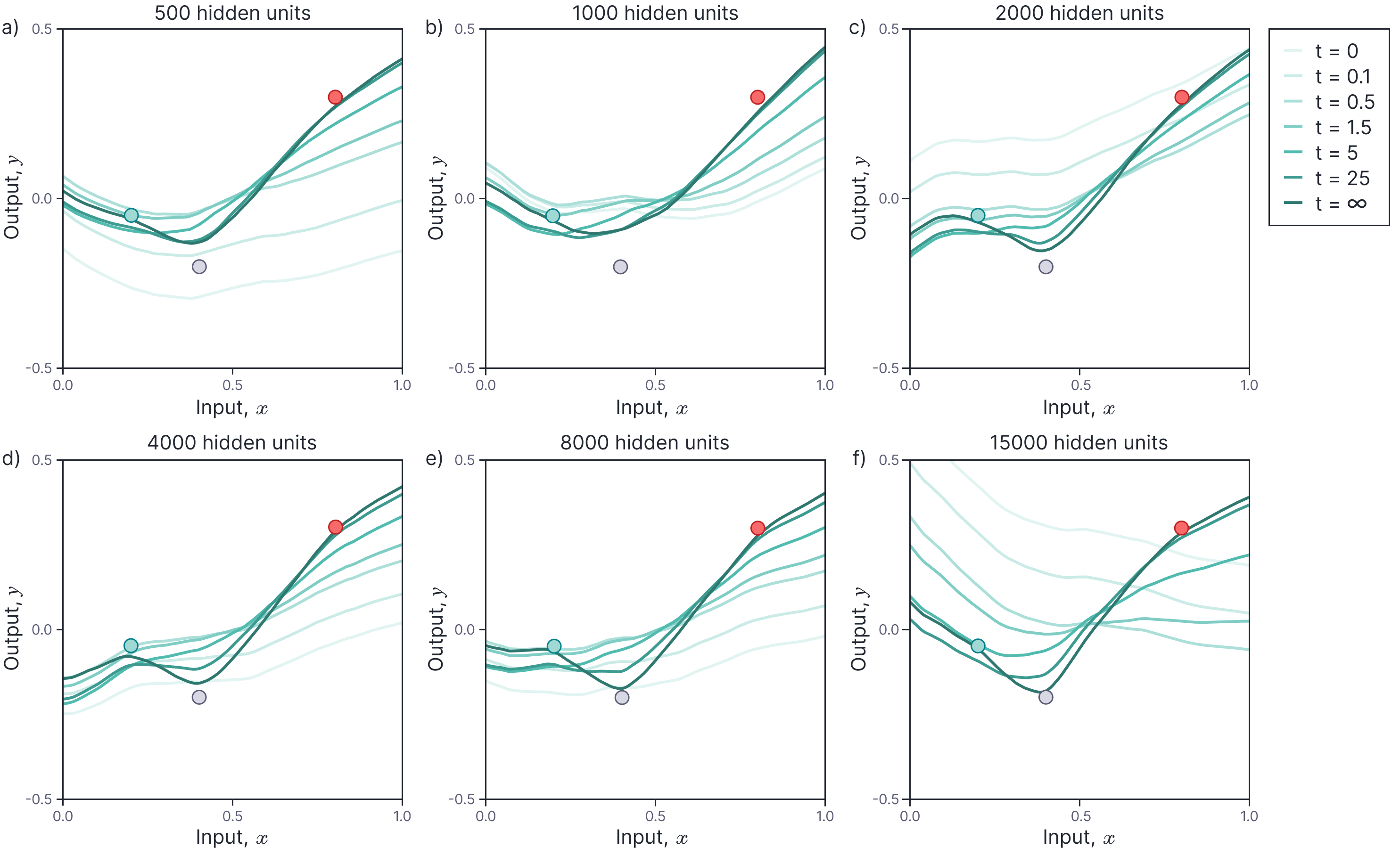
Figure 4 continues the example from figure 1. We visualize the evolution of the predictions over time for randomly initialized shallow networks with different widths.

The predictions of the model improve over time. However, at smaller widths, they do not exactly fit the training points. At first sight, this seems in contradiction to figure 1 where we showed the residuals decrease to zero. This discrepancy can be explained by the fact that the evolution of the parameters $\boldsymbol\phi_{t}$ assumes a linear approximation based on a Taylor series, but equation 14 uses the non-linear neural network model.

Evolution of linearized predictions

Now let’s examine what happens if we use the linear model to make the prediction for a new point $\mathbf{x}^*$:

\begin{equation}
y^* =
\mathbf{ f}[\mathbf{x^*},\boldsymbol\phi_0] + \frac{\partial
\mathbf{ f}[\mathbf{x^*},\boldsymbol\phi_0]}{\partial \boldsymbol\phi}^T\bigl(\boldsymbol\phi-\boldsymbol\phi_{0}\bigr),
\tag{15}
\end{equation}

From equation 13, we have:

\begin{eqnarray}
\boldsymbol\phi_t\!-\!\boldsymbol\phi_0&=& \frac{\partial
\mathbf{ f}[\mathbf{X},\boldsymbol\phi_0]}{\partial \boldsymbol\phi}
\mathbf{ NTK}\bigl[\mathbf{X},\mathbf{X}\bigr]^{-1}\biggl(\mathbf{I}\!-\!\exp\Bigl[-
\mathbf{ NTK}\bigl[\mathbf{X},\mathbf{X}\bigr]\cdot t\Bigr]\biggr) \Bigl(\mathbf{y}\!-\!
\mathbf{ f}[\mathbf{X},\boldsymbol\phi_0]\Bigr),\nonumber
\tag{16}
\end{eqnarray}

and combining these relations, we can make a prediction using the expression:

\begin{eqnarray}\label{eq:NTK3:prediction_evo}
y^* &=&
\mathbf{ f}[\mathbf{x^*},\boldsymbol\phi_0] +
\mathbf{ NTK}\bigl[\mathbf{x}^*,\mathbf{X}\bigr]
\mathbf{ NTK}\bigl[\mathbf{X},\mathbf{X}\bigr]^{-1}\\&&\hspace{3cm}\biggl(\mathbf{I}-\exp\Bigl[-
\mathbf{ NTK}\bigl[\mathbf{X},\mathbf{X}\bigr]\cdot t\Bigr]\biggr) \Bigl(\mathbf{y}-
\mathbf{ f}[\mathbf{X},\boldsymbol\phi_0]\Bigr).\nonumber
\tag{17}
\end{eqnarray}

Figure 5 continues the example from figure 1 and compares the predictions made by:

The latter case is particularly interesting. In the infinite width limit, the model becomes linear and so there is no discrepancy between using the full and linear models. Here, we have initialized the training from the same place as the finite width network, but more naturally, it would start from its expected value of zero.

Initial gradients

If we take the time derivative of the evolution of the predictions (equation 18), we can find the initial direction of gradient descent.

\begin{eqnarray}\label{eq:NTK32:prediction_evvo}
\frac{dy^*}{dt}\biggr|_{t=0} \!\! &\!\!=\!\!&\!\! \frac{d}{dt}\biggl[
\mathbf{ f}[\mathbf{x^*},\boldsymbol\phi_0] +
\mathbf{ NTK}\bigl[\mathbf{x}^*,\mathbf{X}\bigr]
\mathbf{ NTK}\bigl[\mathbf{X},\mathbf{X}\bigr]^{-1}\nonumber\\&&\hspace{2cm}\biggl(\mathbf{I}-\exp\Bigl[-
\mathbf{ NTK}\bigl[\mathbf{X},\mathbf{X}\bigr]\cdot t\Bigr]\biggr) \Bigl(\mathbf{y}-
\mathbf{ f}[\mathbf{X},\boldsymbol\phi_0]\Bigr)\biggr]\biggr|_{t=0}.\nonumber\\
&=&
\mathbf{ NTK}\bigl[\mathbf{x}^*,\mathbf{X}\bigr]\Bigl(\mathbf{y}-
\mathbf{ f}[\mathbf{X},\boldsymbol\phi_0]\Bigr)\nonumber \\
&=& \sum_{i=1}^{I}
\mathbf{ NTK}\bigl[\mathbf{x}^*,\mathbf{x}_{i}\bigr]\Bigl(y_i-
\mathbf{ f}[\mathbf{x}_i,\boldsymbol\phi_0]\Bigr)
\tag{18}
\end{eqnarray}

This tells us that the $i^{th}$ row of the neural tangent $
\mathbf{ NTK}\bigl[\mathbf{x}^*,\mathbf{X}\bigr]$ determines the magnitude of the initial change of the predictions due to the $i^{th}$ residual $y_i-\mbox{f}[\mathbf{x}_{i},\boldsymbol\phi_{0}]$ at the start of training.

Figure 6 visualizes the analytical NTK for an infinitely wide network with a single hidden layer using ReLU activations (see part II of this series of blogs for mathematical formulation). The mathematical formulation for $\mbox{NTK}[\mathbf{x}^*,\mathbf{x}]$ depends on the angle between arguments $\mathbf{x}^*$ and $\mathbf{x}$ and so this is plotted for $\mathbf{x}^*,\mathbf{x}\in\mathbb{R}^2$. In each panel, the cyan point represents $\mathbf{x}$ and the heatmap represents the value of the neural tangent kernel for every $\mathbf{x}^*$. As discussed in the previous section, the heatmap can be interpreted as the initial change in the predictions at each $\mathbf{x}^*$ induced due to a residual error in the training data at the point $\mathbf{x}$.

Inspection of figure 6 reveals that the kernel has a structure that depends on the radial angle between the points. Considering points on the unit circle (white circle), the kernel response falls off symmetrically as the angular distance between $\mathbf{x}$ and $\mathbf{x}^*$ decreases (as visualized in this video). However, since it is usual to append the value 1 to the inputs to incorporate biases at the first hidden layer, one dimensional inputs $x^*$ and $x$ would lie on the horizontal cyan line in this plot. The values along this line in the three panels represent the kernel value for $x^*\in[-4,4]$ for values $x=0,1,3$ respectively. In accordance with equation 18, the profiles along these line would determine the initial changes in the output function due to training points at positions $x=0,1,3$.

Kernel regression

Equation 18 describes the training evolution of the neural network. In the infinite width limit at $t=\infty$, the expected output with the initial parameters is zero and the exponential term disappears, so we can make predictions using:

\begin{eqnarray}\label{eq:NTK3:kernel_regression}
y^* =
\mathbf{NTK}\bigl[\mathbf{x}^*,\mathbf{X}\bigr]
\mathbf{ NTK}\bigl[\mathbf{X},\mathbf{X}\bigr]^{-1} \mathbf{y}.\nonumber
\end{eqnarray}

where the neural tangent kernels are computed analytically as described in part II of this series of articles. This approach is known as kernel regression and is quite surprising; we can compute the prediction for an infinite width network without ever training the network, or even explicitly evaluating it.

This seems extremely convenient, but unfortunately it has two major disadvantages. First, the inverse NTK term is size $ID_{out}\times ID_{out}$ where $I$ is the number of training examples and $D_{out}$ is the number of network outputs (classes for a classification task). Consequently, evaluating this expression is only practical for relatively small datasets.

Second, the performance of kernel methods is generally inferior to that for training neural networks in the conventional way. For example, Arora et al. 2019 found that performance on CIFAR-10 was almost 5% less with a kernel method even after batch norm and data augmentation were removed (adding these would increase the gap). One possible explanation for this discrepancy is that performance is improved in the standard setting by implicit regualarization due to stochastic gradient descent. Subsequent work (e.g., Li et al. 2019) has partially bridged this gap, but kernel methods still do not generally perform as well as the standard method of training neural networks.

NTK Gaussian processes

We can rewrite the formula for the evolution of the predictions (equation 18) as an affine transformation of the initial network outputs:

\begin{eqnarray}\label{eq:NTK3:NTK_GP}
y^* \!\! &\!\!=\!\!&\!\!
\mathbf{f}[\mathbf{x^*},\boldsymbol\phi_0] +
\mathbf{ NTK}\bigl[\mathbf{x}^*,\mathbf{X}\bigr]
\mathbf{ NTK}\bigl[\mathbf{X},\mathbf{X}\bigr]^{-1}\nonumber \\&&\hspace{3cm}\Bigl(\mathbf{I}-\exp\Bigl[-
\mathbf{NTK}\bigl[\mathbf{X},\mathbf{X}\bigr]\cdot t\Bigr]\Bigr) \Bigl(\mathbf{y}-
\mathbf{ f}[\mathbf{X},\boldsymbol\phi_0]\Bigr)\nonumber\\
&\!\!=\!\!&\!\!
\mathbf{ NTK}\bigl[\mathbf{x}^*,\mathbf{X}\bigr]
\mathbf{ NTK}\bigl[\mathbf{X},\mathbf{X}\bigr]^{-1}\Bigl(\mathbf{I}-\exp\Bigl[-
\mathbf{ NTK}\bigl[\mathbf{X},\mathbf{X}\bigr]\cdot t\Bigr]\Bigr) \mathbf{y}\nonumber\\
&&\hspace{0.0cm}\!+\!\Bigl[1, –
\mathbf{ NTK}\bigl[\mathbf{x}^*,\mathbf{X}\bigr]
\mathbf{ NTK}\bigl[\mathbf{X},\mathbf{X}\bigr]^{-1}\Bigl(\mathbf{I}\!-\!\exp\Bigl[-
\mathbf{ NTK}\bigl[\mathbf{X},\mathbf{X}\bigr]\cdot t\Bigr]\Bigr) \Bigr]\begin{bmatrix}
\mathbf{ f}[\mathbf{x^*},\boldsymbol\phi_0] \\
\mathbf{ f}[\mathbf{X},\boldsymbol\phi_0]\end{bmatrix}\nonumber \\
&=& a + \mathbf{b}\begin{bmatrix}
\mathbf{ f}[\mathbf{x^*},\boldsymbol\phi_0] \\
\mathbf{ f}[\mathbf{X},\boldsymbol\phi_0]\end{bmatrix}.
\tag{19}
\end{eqnarray}

The initial network outputs $\mathbf{f}[\mathbf{x^*},\boldsymbol\phi_0]$ and $\mathbf{f}[\mathbf{X},\boldsymbol\phi_0]$ are jointly Gaussian distributed for an infinite width network with normally distributed parameters, and so we can use the relation (see proof at end of part I of this blog) that if $Pr(\mathbf{z})= \mbox{Norm}_{\mathbf{z}}[\boldsymbol\mu, \boldsymbol\Sigma]$, then the affine transform $\mathbf{a}+\mathbf{B}\mathbf{z}$ is distributed as:

\begin{equation}
Pr(\mathbf{a}+\mathbf{B}\mathbf{z}) = \mbox{Norm}\Bigl[\mathbf{a} + \mathbf{B} \boldsymbol\mu, \mathbf{B}\boldsymbol\Sigma\mathbf{B}^{T}\Bigr].
\tag{20}
\end{equation}

In this way, we can compute not only the evolution of the average prediction for input $\mathbf{x}^{*}$ but also the uncertainty in that prediction. This is known as a neural tangent kernel Gaussian process (see Lee et al., 2019).

For an infinite width shallow ReLU network with normally distributed weights with mean zero and prior variance $\sigma^{2}_p$, the mean of the initial outputs is $\boldsymbol\mu=0$ and element $i,j$ of the covariance matrix $\boldsymbol\Sigma$ can be shown (non-obviously) to be:

\begin{equation}
\boldsymbol\Sigma_{ij} = \sigma_{p} \lVert\mathbf{x}_{i}\rVert\lVert\mathbf{x}_{j}\rVert \frac{(\pi-\theta)\cos[\theta]+\sin[\theta]}{2\pi} +1,
\tag{21}
\end{equation}

where $\theta$ is the angle between the two inputs:

\begin{equation}
\theta = \arccos\left[\frac{\mathbf{x}_{i}^{T}\mathbf{x}_{j}}{\lVert\mathbf{x}_{i}\rVert\lVert\mathbf{x}_{j}\rVert}\right].
\tag{22}
\end{equation}

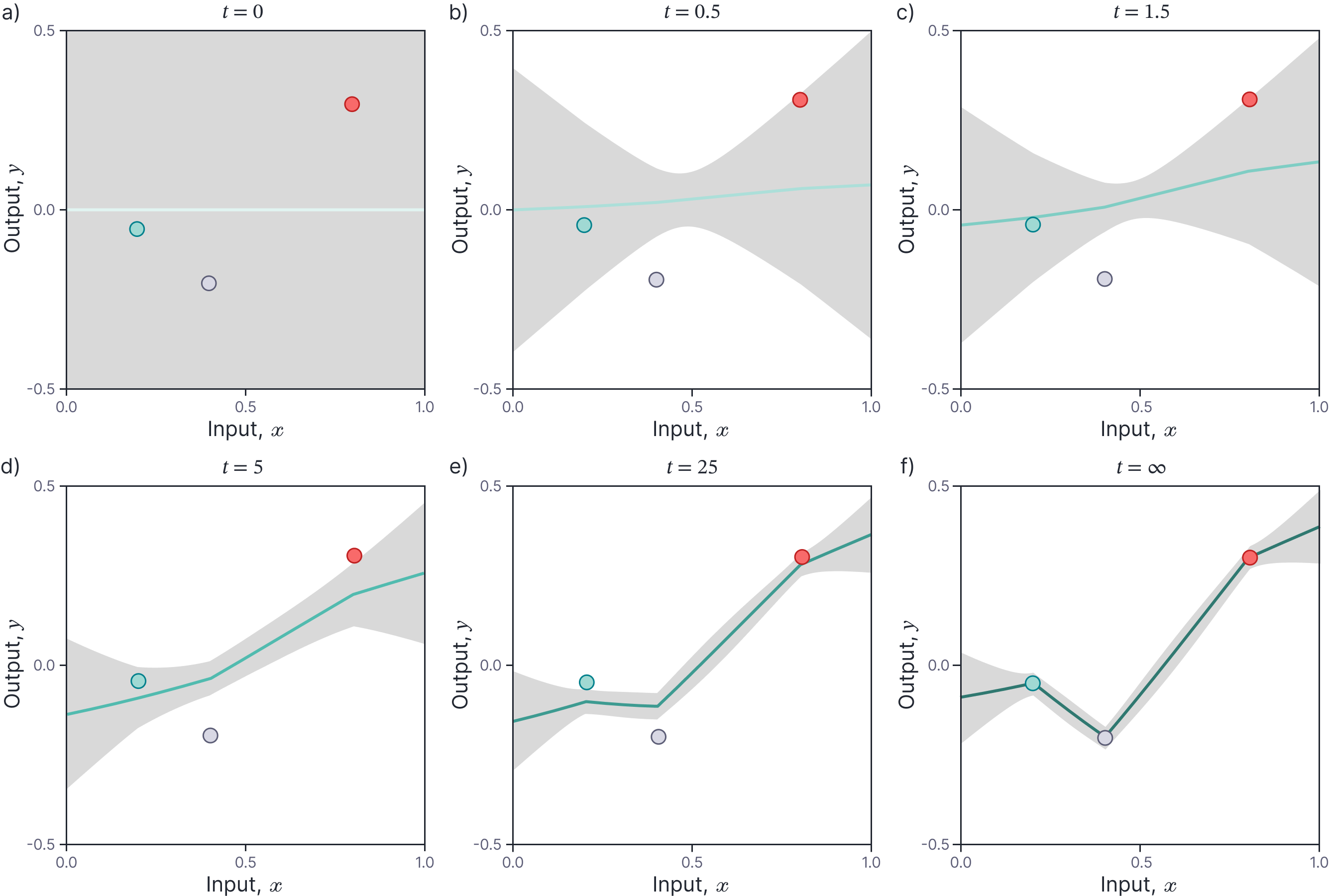
Figure 7 shows the evolution of the uncertainty as a function of time as we fit a neural network to the three points in our working example. By convention, we add a small noise term $\sigma^{2}$ to the output to account for measurement noise.

The NTK and generalizability

Finally, we note that since the predictions of the network are governed by the NTK (equation 19), it has also been used to provide insights about the generalization of networks. For example, Geiger et al. (2020) exploit the NTK to predict the decrease in error found in the overparameterized regime of the double descent curve. The explain this decrease in error in terms of a decreases in random fluctuations in the output function due to initialization as the capacity increases. A different strand of work has identified the condition number of the NTK as predicting generalization ability (Xiao et al., 2018; Xiao et al., 2020). This has led other authors to exploit the NTK for architecture search (Park et al., 2020; Chen et al. (2021)).

Conclusion

This series of blogs has explored gradient flow and the NTK. In part I we considered the properties of gradient flow in linear models. In part II, we showed that neural networks become linear in the infinite width limit and so these properties are applicable. This led to the development of the neural tangent kernel.

In this third part, we have explored the implications of the NTK. We have shown that the NTK provides information about trainability and convergence speed in infinite width networks and that bounds can be derived for finite width networks. Furthermore, the NTK allows us to write closed form expressions for the evolution of the parameters and predictions, and their uncertainty. The initial changes in the predictions to be decomposed into a linear sum of contributions from each training point, where this decomposition depends on the NTK. In addition, the NTK can be used to make network predictions without ever training the network and to partially predict the generalizability of networks without ever training them.

*The code related to this blog post can be found on github here.