
Introduction
In December 2019, many Borealis employees travelled to Vancouver to attend NeurIPS 2019. With almost 1500 accepted papers, there’s a lot of great work to sift through. In this post, some of our researchers describe the papers that they thought were especially important.
Latent ODEs for irregularly-sampled time-series
Yulia Rubanova, Ricky T. Q. Chen, David Duvenaud
by Alex Radovic
Related Papers:
What problem does it solve? It is a new neural network architecture optimized for irregularly-sampled time series.
Why this is important? Real world data is often sparse and/or irregular in time. For example, sometimes data is recorded when a sensor updates in response to some external stimulus, or an agent decides to make a measurement. The timing of these data points can itself be a powerful predictor, so we would like a neural network architecture that is designed to extract that signal.
Zero padding and other approaches are sometimes used so that a simple LSTM or GRU can be applied. However, this makes for a less efficient and sparser data representation that those recurrent networks are not well equipped to deal with.
The approach taken and how it relates to previous work: Neural ODEs are only a year old but are paving the way for a number of fascinating applications. Neural ODEs reinterpret repeating neural network layers as approximations to a differential equation expressed as a function of depth. As pointed out in the original paper, a Neural ODE can also be a function of some variable of interest (e.g., time).
The original Neural ODE paper does touch on potential uses for time series data, and uses a Neural ODE to generate time series data. This paper describes a modified RNN that has a hidden state that changes both when a new data point comes in and as a function of time between observations. The architecture is a development of a well explored idea where the hidden state decays as some function of time between observations (Cao et al., 2018; Mozer et al., 2017; Rajkomar et al., 2018; Che et al., 2018). Now instead of a preset function, the hidden state between observations is the solution to a Neural ODE. Figure 1 shows how information is updated in an ODE-RNN in contrast to other common approaches.
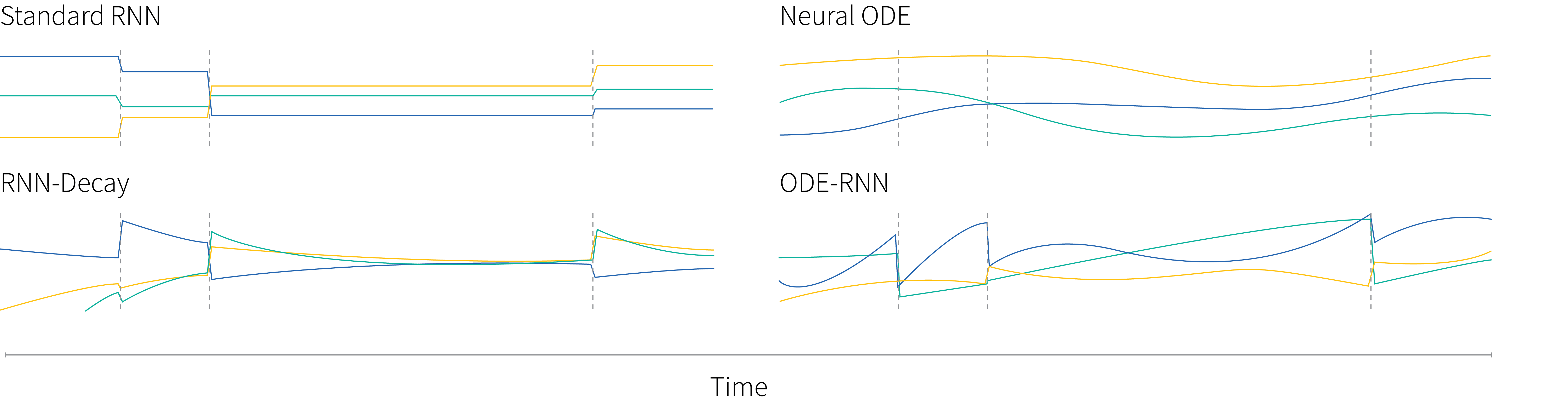
Figure 1. Trajectories of hidden states. Each line shows one dimension of the hidden state. Each vertical jump denotes an observation. Standard RNNs only change when there is an observation. The RNN decay model gradually decays after each observation. Hidden states in the original neural-ODE model have a complex trajectory but these do not depend on observations. The ODE-RNN model has states that have complex trajectories, but react to observations.
Results: They show state of the art performance at both interpolation and extrapolation on MuJoCo simulation and the PhysioNet datasets. The PhysioNet dataset is particularly exciting as it represents an important real world scenario consisting of patients’ intensive care unit data. The extrapolation is particularly impressive as successful interpolation methods often don’t extrapolate well. Figure 2 shows on a toy dataset how using an ODE-RNN encoder rather than an RNN encoder leads to much better extrapolation in the ODE decoder.
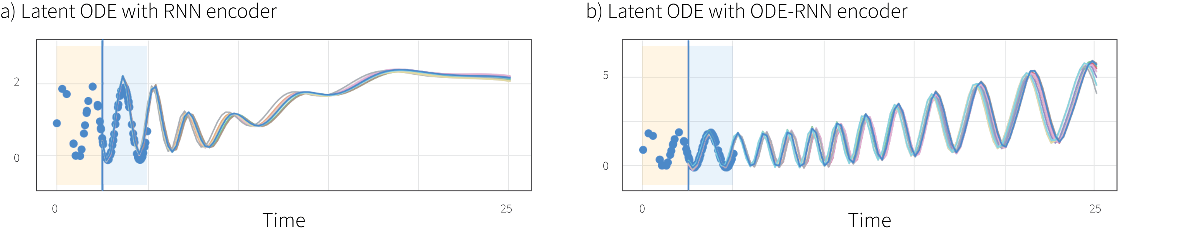
Figure 2. Approximate posterior samples conditioned on 20 points in the yellow region. a) Latent ODE model conditions on yellow area and reconstructs in blue area but does not manage to extrapolate sensibly. b) ODE-RNN network conditions on yellow area and solves ODE over large time interval. The resulting samples are much more plausible predictions.
Selective sampling-based scalable sparse subspace clustering (S$^5$C)
Shin Matsushima, Maria Brbić
Related Papers:
What problem does it solve? High-dimensional data (e.g., videos, text) often lies on a low dimensional manifold. Subspace clustering algorithms such as the Sparse Subspace Clustering (SSC) algorithm assume that this manifold can be approximated by a union of lower dimensional subspaces. Such algorithms try to identify these subspaces and associate them with individual data points. This paper improves the speed and memory cost of the SSC algorithm while retaining theoretical guarantees by introducing an algorithm called Selective Sampling-based Scalable Sparse Subspace Clustering (S$^5$C).
Why this is important? The method scales to large datasets which was a big practical limitation of the SSC algorithm. It also comes with theoretical guarantees and these empirically translate to improved performance.
Previous Work: The original SSC algorithm consisted of two steps: representation learning and spectral clustering . The first step learns an affinity matrix $\mathbf{W}$. Intuitively the $ij$-components of $\mathbf{W}$ encodes the “similarity” between point $i$ and $j$ (but with $W_{ii} = 0$ for all $i$). The matrix $\mathbf{W} = |\mathbf{C}| + |\mathbf{C}|^T$ is made sparse by imposing an $\ell_1$ norm regularizer on the objective functions:
\begin{equation}\label{eq:sccobjective}\underset{\left(C_{j i}\right)_{j \in[N]} \in \mathbb{R}^{N}}{\operatorname{minimize}} \frac{1}{2}\left\|\mathbf{x}_{i}-\sum_{j \in[N]} C_{j i} \mathbf{x}_{j}\right\|_{2}^{2}+\lambda \sum_{j \in[N]}\left|C_{j i}\right|, \text { subject to } C_{i i}=0. \tag{1}\end{equation}
where $\mathbf{x}_i \in \mathbb{R}^M$ is a data point in the dataset and the $N$ different objective functions determine the $N$ rows of $\mathbf{C}$.
This $\ell_1$ regularizer should not affect the ability of $\mathbf{W}$ to minimize the unregularized objective if the data points lie in subspaces that are of lower dimensions than the original embedding space. The regularization will produce a $\mathbf{W}$ whose non-zero elements suggests that the linked data points are within the same subspace.
The second step of the SSC algorithm applies spectral clustering to $\mathbf{W}$. The eigenvectors of the Laplacian $\mathbf{L} = \mathbf{I} – \mathbf{D}^{-1/2}\mathbf{W}\mathbf{D}^{-1/2}$ are computed, where $\mathbf{D}$ is a diagonal matrix with $D_{ii} = \sum_j W_{ij}$. For $N_{c}$ clusters, the eigenvectors associated with the with $N_{c}$ smallest non-zero eigenvalues are chosen, normalised, and stacked into a matrix $\mathbf{X} \in \mathbb{R}^{N\times N_c }$. Each row represents a data point and their cluster memberships are determined by further clustering in this $\mathbb{R}^{N_c}$ space using k-means.
Many other approaches aim to improve SSC. Some algorithms like OMP (Dyer et al., 2013; You and Vidal 2015), PIC (Lin and Cohen, 2010), and nearest neighbor SSC (Park et al., 2014) retain theoretical guarantees but still suffer from scalability issues. Other fast methods such as EnSC-ORGEN (You et al., 2013), and SSSC (Peng et al., 2013) exist at the expense of theoretical guarantees and justification.
Approach taken: Each of the $N$ components of the objective function in equation 1 has $O(N)$ parameters. The minimization procedure can be done in a time and space complexity of $O(N^2)$, so this does not scale to well in $N$. Instead S$^5$C aims to solve $N$ problems having $T$ parameters by selecting $T$ vectors that can be used to represent the rest of the dataset. The intuition is that data points from each subspace can be reconstructed from the span of a few selected vectors denoted by the set $\mathcal{S}$. The vectors in $\mathcal{S}$ are selected incrementally by stochastic approximation of a sub-gradient; a subsample $I\subset [N]$ (with $|I| \ll N$) of vectors of the full dataset are selected and used to estimate which data point in $[N]$ best improves the data representation spanned by $\mathcal{S}$. This step has $\mathcal{O}(\left|I\right|N)$ complexity. This step repeated $T$ times to build $\mathcal{S}$, giving a complexity of $\mathcal{O}(\left|I\right|TN)$ instead of $\mathcal{O}(N^3)$ to build the affinity matrix $\mathbf{W}$. This construction ensures that $\mathbf{W}$ only has $\mathcal{O}(N)$ non-zero elements and hence the eigenvector decomposition can also be done in $\mathcal{O}(N)$ time using orthogonal iteration.
Results: Figure 3 shows the linear increase in time as a function of dataset size. Figure 4 shows improvements on the clustering error on many datasets when comparing to other fast algorithms without theoretical guarantees.
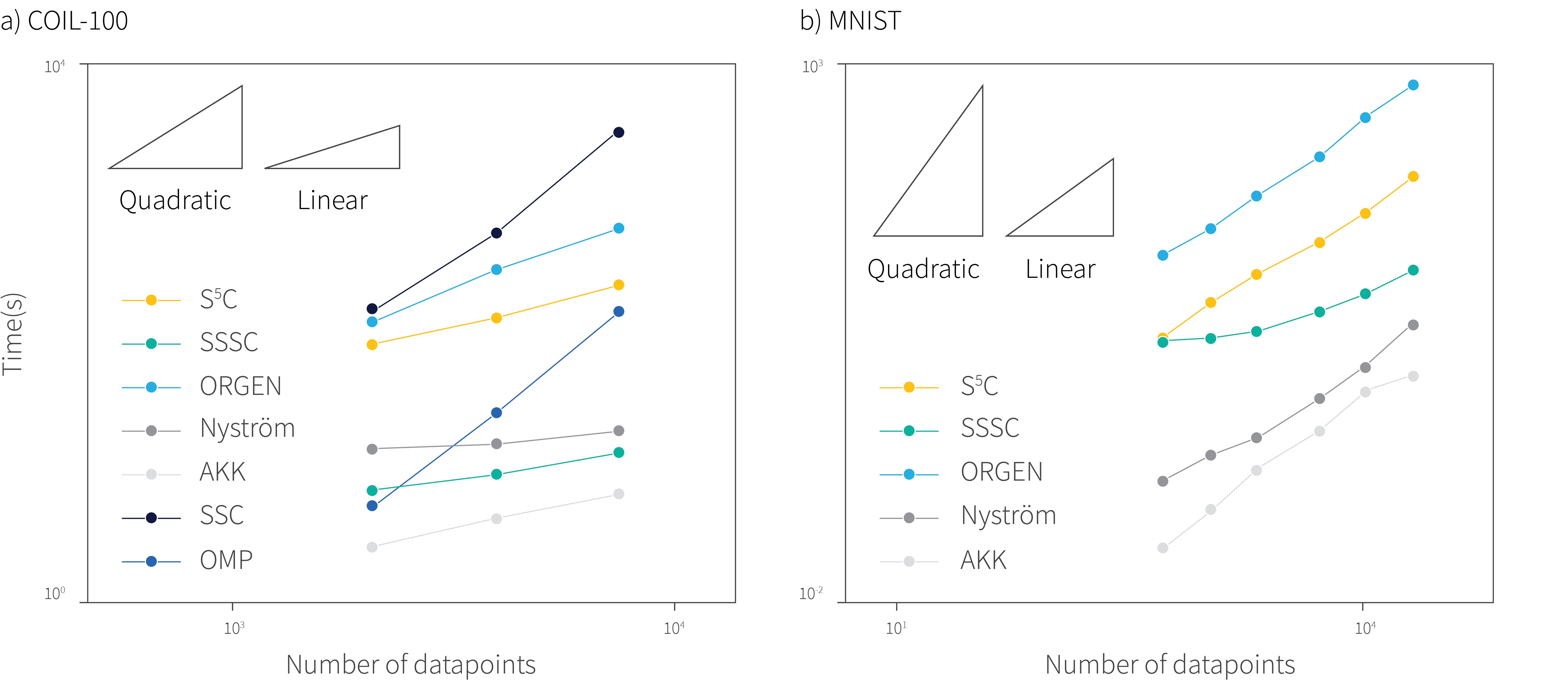
Figure 3. Time scaling of various clustering algorithms as a function of dataset size for two datasets COIL-100 and MNIST.
| Dataset | Nyström | dKK | SSC | SSC-OMP | SSC-ORGEN | SSSC | S5C |
|---|---|---|---|---|---|---|---|
| Yale B | 76.8 | 85.7 | 33.8 | 35.9 | 37.4 | 59.6 | 39.3 (1.8) |
| Hopkins 155 | 21.8 | 20.6 | 4.1 | 23.0 | 20.5 | 21.1 | 14.6 (0.4) |
| COIL-100 | 54.5 | 53.1 | 42.5 | 57.9 | 89.7 | 67.8 | 45.9 (0.5) |
| Letter-rec | 73.3 | 71.7 | / | 95.2 | 68.6 | 68.4 | 67.7 (1.3) |
| CIFAR-10 | 76.6 | 75.6 | / | / | 82.4 | 82.4 | 75.1 (0.8) |
| MNIST | 45.7 | 44.6 | / | / | 28.7 | 48.7 | 40.4 (2.3) |
| Devanagari | 73.5 | 72.8 | / | / | 58.6 | 84.9 | 67.2 (1.3) |
Figure 4. Clustering error in $\%$. Error bars (if available) are in parentheses. Experiments where a time limit of 24 hours or memory limit of 16 GB was exceeded are denoted by $/$.
Graph Normalizing Flows
Jenny Liu, Aviral Kumar, Jimmy Ba, Jamie Kiros, Kevin Swersky
Related Papers:
What problem does it solve? It introduces a new invertible graph neural network that can be used for supervised tasks such as node classification and unsupervised tasks such as graph generation.
Why this is important? Graph representation learning has diverse applications from bioinformatics to social networks and transportation. It is challenging due to diverse possible representations and complex structural dependencies among nodes. In recent years, graph neural networks have been the state-of-the-art model for graph representation learning. This paper proposes a new graph neural model with less memory footprint, better scalability, and room for parallel computation. Additionally, this model can be used for graph generation.
The approach taken and how it relates to previous work: The model builds on both message passing in graph neural networks and normalizing flows. The idea is to adapt normalizing flows for node feature transformation and generation.
Given a graph with $N$ nodes and node features $\mathbf{H} \in \mathbb{R}^{N \times d_n}$, graph neural networks transform the raw features $\mathbf{H}$ to embedded features that capture the contextual and structural information of the graph. This transformation consists of a series of message passing steps, where step $t$ consists of i) message generation using function $\mathbf{M}_t[\bullet]$ and ii) updating the node features with the aggregated messages of the neighboring nodes using function $\mathbf{U}_t[\bullet]$:\begin{align}\label{message-passing}
&\mathbf{m}_{t+1}^{(v)} = \mathbf{Agg}\left[\{\mathbf{M}_t[\mathbf{h}_{t}^{(v)}, \mathbf{h}_{t}^{(u)}]\}_{u \in \mathcal{N}_v}\right] \nonumber\\
&\mathbf{h}_{t+1}^{(v)} = \mathbf{U}_t[\mathbf{h}_{t}^{(v)}, \mathbf{m}_{t+1}^{(v)}]. \tag{2}
\end{align}
Normalizing flows are generative models which find an invertible mapping $\mathbf{z}=\mathbf{f}[\mathbf{x}]$ to transform the data $\mathbf{x}$ to a latent variable $\mathbf{z}$ with a simple prior distribution (e.g., $\mbox{Norm}_{\mathbf{z}}[\mathbf{0}, \mathbf{I}]$). By sampling $\mathbf{z}$ and applying the inverse function $\mathbf{f}^{-1}[\bullet]$, we can generate data from the target distribution. This paper is based on the RealNVP which uses the mapping:\begin{align}\label{realnvp_map}
\mathbf{z}^{(0)}&= \mathbf{x}^{(0)} \exp{\left[\mathbf{f}_1\left[\mathbf{x}^{(1)}\right]\right]} + \mathbf{f}_2\left[\mathbf{x}^{(1)}\right] \nonumber\\
\mathbf{z}^{(1)}&=\mathbf{x}^{(1)},\nonumber
\end{align}
where $\mathbf{x}^{(0)}$ and $\mathbf{x}^{(1)}$ are partitions of the input $\mathbf{x}$, and the output $\mathbf{z}$ is obtained by concatenating $\mathbf{z}^{(0)}$ and $\mathbf{z}^{(1)}$. The functions $\mathbf{f}_1[\bullet]$ and $\mathbf{f}_2[\bullet]$ are neural networks. RealNVP cascades these mapping functions with random partitioning at each step.
This paper extends normalizing flows to graphs by applying the RealNVP mapping functions to the node feature matrix $\mathbf{H}$ (figure 5a):
\begin{align}\label{realnvp_graph} \mathbf{H}_{t+1}^{(0)}&= \mathbf{H}_{t}^{(0)} \exp{\left[\mathbf{F}_1\left[\mathbf{H}_{t}^{(1)}\right]\right]} + \mathbf{F}_2\left[\mathbf{H}_{t}^{(1)}\right] \nonumber\\
\mathbf{H}_{t+1}^{(1)}&=\mathbf{H}_{t}^{(1)},\nonumber
\end{align}
where the functions $\mathbf{F}_1[\bullet]$ and $\mathbf{F}_2[\bullet]$ can be any message-based transformation and are chosen here to be graph attention layers. In practice, an alternating pattern is used for consecutive operations.
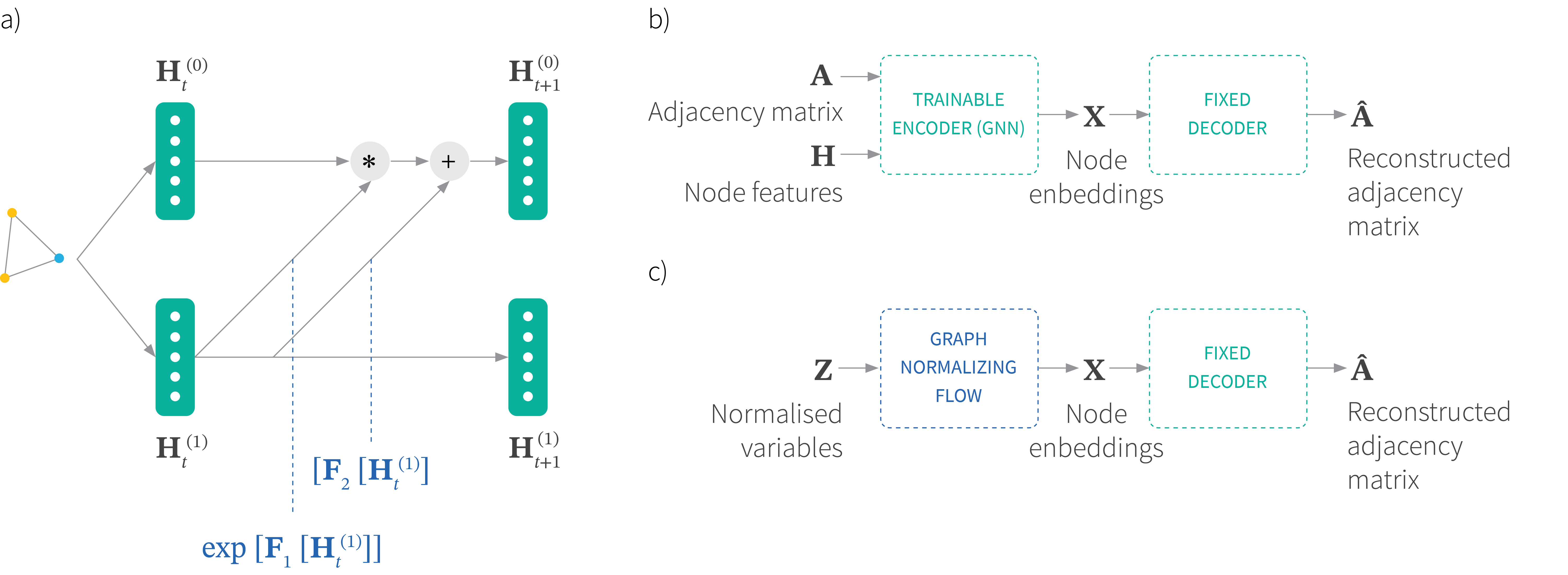
Figure 5. a) Invertible message passing transformation for graph normalizing flows. The feature matrix $\mathbf{H}$ is partitioned into two subsets of feature dimensions. An affine coupling flow relates the feature at step $t$ to step $t+1$. b) To generate a new random graph, an autoencoder is first trained that takes an adjacency matrix $\mathbf{A}$ and a set of node features $\mathbf{H}$ and produces a node embedding $\mathbf{X}$ from which the adjacency matrix can be reconstructed. c) Then a graph normalizing flow is trained to generate these embeddings, which be converted to new adjacency matrices via the decoder.
In the supervised setting, the raw features are transformed through these layers to perform downstream tasks such as node classification. The resulting network is called GRevNet. Ordinary graph neural networks need to store the hidden states after each message passing step to do backpropagation. However, the reversible functions of GRevNet can save memory by reconstructing the hidden states in the backpropagation phase.
In addition, the graph normalizing flow can generate graphs via a two step process. First, a permutation-invariant graph autoencoder is trained to encode the graph to continuous node embeddings $\mathbf{X}$ and use these to reconstruct the adjacency matrix (figure 5b). Here, the encoder is a graph neural network and the decoder is a fixed function that makes nodes adjacent if their respective columns of $\mathbf{X}$ are similar. Second, a graph normalizing flow is trained to map from $\mathbf{z} \sim \mbox{Norm}_[\mathbf{0},\mathbf{I}]$ to a target distribution of node embeddings $\mathbf{X} \in \mathbb{R}^{N \times d_e}$. We generate from this distribution and use the decoder to generate new adjacency matrices (figure 5c).
Results: In a supervised context, GRevNet is used to classify documents (on Cora and Pubmed dataset) and protein-protein interaction (on PPI dataset) and compares favorably with other approaches. In the unsupervised context, the GNF model is used for graph generation on two datasets, COMMUNITY-SMALL and EGO-SMALL and is competitive with the popular GraphRNN.
R2D2: Repeatable and reliable detector and descriptor
Jerome Revaud, Philippe Weinzaepfel, César De Souza, Martin Humenberger
by Jimmy Chen
Related Papers:
What problem does it solve? Keypoints are pixel locations where local image patches are quasi-invariant to camera viewpoint changes, photometric transformations, and partial occlusion. The goal of this paper is to detect keypoints and extract visual feature vectors from the surrounding image patches.
Why this is important? Keypoint detection and local feature description are the foundation of many applications such as image matching and 3D reconstruction.
The approach taken how it relates to previous work: R2D2 proposes a three-branch network to predict keypoint reliability, repeatability and image patch descriptors simultaneously (figure 6). Repeatability is a measure of the degree to which a keypoint can be detected at different scales, under different illuminations, and with different camera angles. Reliability is a measure of how easily the feature descriptor can be distinguished from others. R2D2 proposes a learning process that improves both repeatability and reliability.
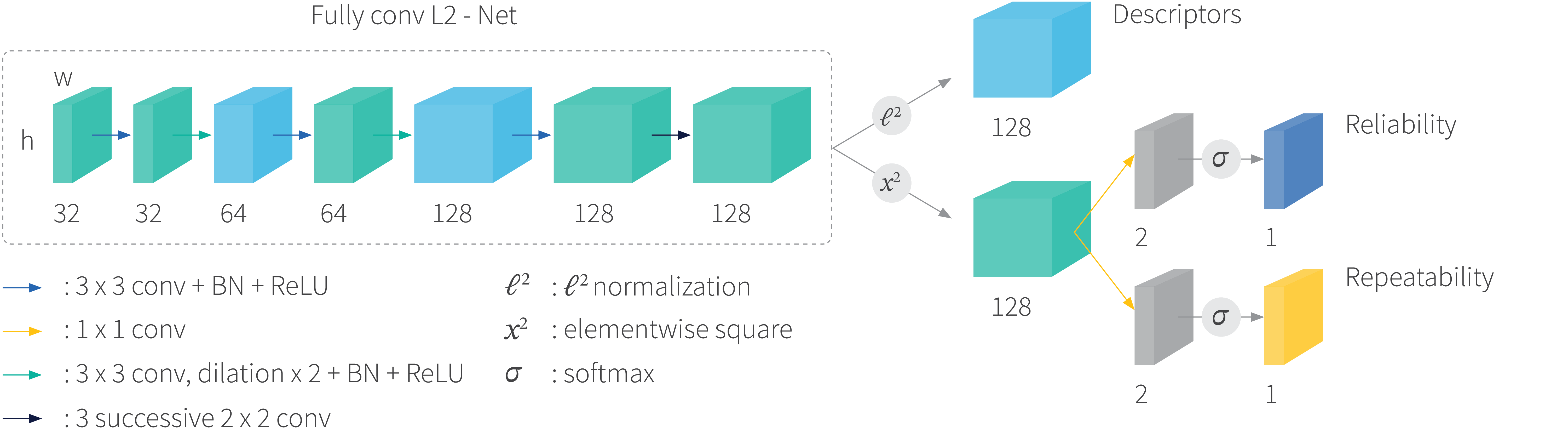
Figure 6. The R2D2 network has three branches which compute maps for the descriptors, reliability and repeatability. Each has the same spatial resolution as the input image.
Figure 7 shows a toy example of repeatability and reliability that are predicted by R2D2 in two images. The corners of the triangle in the first image are both repeatable and reliable. The grid corners in the second image are repeatable but not reliable as there are many similar corners nearby.
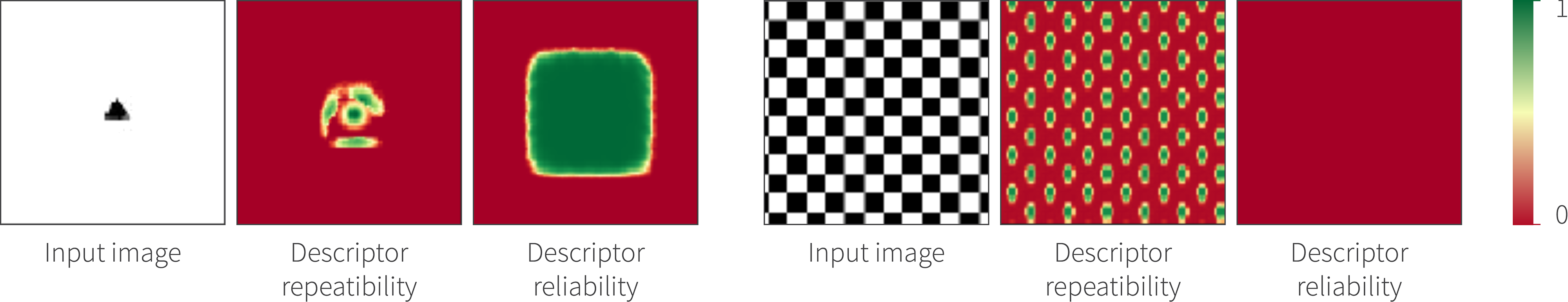
Figure 7. Two examples of keypoint repeatability and reliability. The three columns represent the input image, repeatability and reliability maps. Adapted from Revaut et al. (2019).
Results: R2D2 is tested on the HPatches dataset for image matching. Performance is measured by mean matching accuracy. Figure 8 shows that R2D2 significantly outperforms previous work at nearly all error thresholds. R2D2 is also tested on the Aachen Day-Night dataset for camera relocalization. R2D2 achieves state-of-the-art accuracy with a smaller model size (figure 9). The paper also provides qualitative results and an ablation study.
Although the paper demonstrated impressive results, the audience raised concerns about the keypoint sub-pixel accuracy and computation cost for large images.
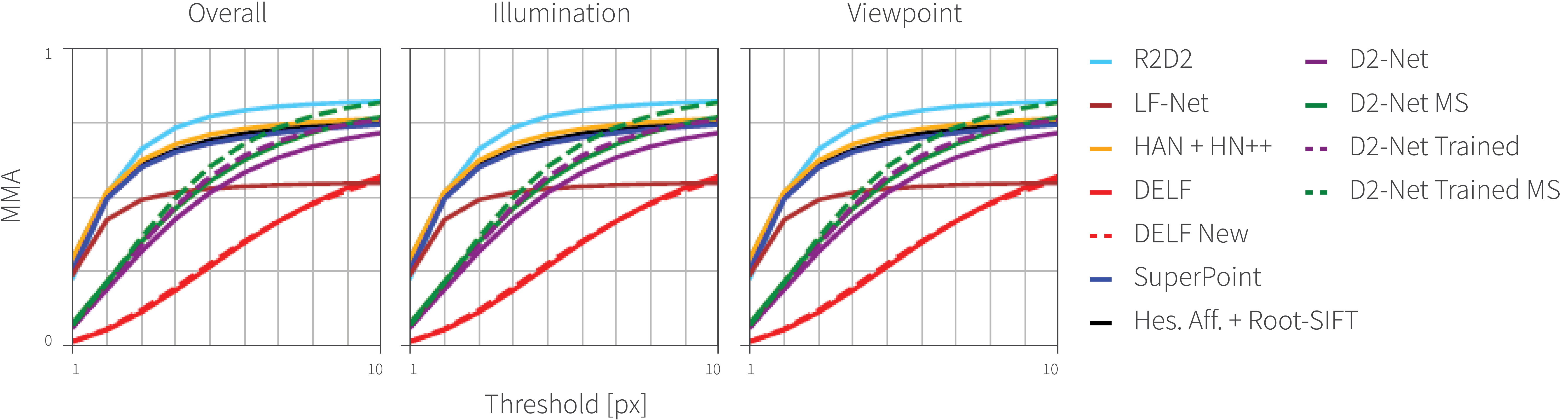
Figure 8. Mean matching accuracy (MMA) on the HPatches dataset. Adapted from Revaut et al. (2019).
| Method | #kpts | dim | #weights | 0.5m, 2° | 1m, 5° | 5m, 10° |
|---|---|---|---|---|---|---|
| RootSIFT [24] | 11K | 128 | – | 33.7 | 52.0 | 65.3 |
| HAN+HN [30] | 11K | 128 | 2 M | 37.8 | 54.1 | 75.5 |
| SuperPoint [9] | 7K | 256 | 1.3 M | 42.8 | 57.1 | 75.5 |
| DELF (new) [32] | 11K | 1024 | 9 M | 39.8 | 61.2 | 85.7 |
| D2-Net [11] | 19K | 512 | 15 M | 44.9 | 66.3 | 88.8 |
| R2D2, $N$ = 16 | 5K | 128 | 0.5 M | 45.9 | 65.3 | 86.7 |
| R2D2 $N$ = 8 | 10K | 128 | 1.0 M | 45.9 | 66.3 | 88.8 |
Figure 9. Results for Aachen Day-Night visual localization task.
Unlabeled data improves adversarial robustness
Yair Carmon, Aditi Raghunathan, Ludwig Schmidt, Percy Liang, John C. Duchi
&
Are labels required for improving adversarial robustness?
Jonathan Uesato, Jean-Baptiste Alayrac, Po-Sen Huang, Robert Stanforth, Alhussein Fawzi, Pushmeet Kohli
What problem do they solve? Both papers incorporate unlabeled data into adversarial training to improve adversarial robustness of neural networks.
Why this is important? We would like to be able to train neural networks in such a way that they are robust to adversarial attack. This is difficult, but we do not fully understand why. It could be that we need to use significantly larger models than we can currently train. Alternatively, it might be that we need a new training algorithm that has not yet been discovered. Another possibility is that adversarially robust networks have a very high sample complexity and so we just don’t use enough data to train a robust model.
These two papers pertain to the latter sample complexity issue. They ask whether we can exploit additional unlabeled data to boost the adversarial robustness of a neural network. Since unlabeled data is relatively abundant this potentially provides a practical way to train adversarially robust models.
The approach taken and how it relates to previous work: We assume that each data-label pair $(\mathbf{x}, y)$ is sampled from distribution $\mathcal{D}$, and we are learning a model $Pr(y|\mathbf{x},\boldsymbol\theta)$ that predicts the probability of the label from the data and has parameters $\boldsymbol\theta$. The standard training objective is
\begin{equation}\min_{\boldsymbol\theta}\left[ \mathbb{E}_{(\mathbf{x}, y)\sim \mathcal{D}}\left[\mbox{xent}\left[y, Pr(y|\mathbf{x},\boldsymbol\theta)\right]\right]\right] \tag{3}\label{eq:clean_training}\end{equation}
where $\mbox{xent}[\bullet, \bullet]$ is the cross-entropy loss.
When we train for adversarial robustness, we want the model to make the same prediction within a neighborhood and we train the model using the min-max formation (Madry et al., 2017):\begin{equation}
\min_{\boldsymbol\theta}\left[ \mathbb{E}_{(\mathbf{x}, y)\sim \mathcal{D}}\left[\max_{\boldsymbol\delta\in B_\epsilon}\left[\mbox{xent}\left[y, Pr(y|\mathbf{x}+\boldsymbol\delta,\boldsymbol\theta)\right]\right]\right]\right] \tag{4}
\label{eq:minmax_training}
\end{equation}
where $B_\epsilon$ is a ball with radius $\epsilon$. In other words, we minimize the maximum cross-entropy loss with in a small neighborhood to achieve robustness.
TRADES improved adversarial training by separating the inner maximization term into a classification loss and a regularization loss:
\begin{equation}\min_\theta \left[\mathbb{E}_{(\mathbf{x}, y)\sim \mathcal{D}}\left[\mbox{xent}\left[y, Pr(y|\mathbf{x},\boldsymbol\theta)\right] + \frac{1}{\lambda}\max_{\boldsymbol\delta\in B_\epsilon}\left[\mbox{D}_{KL}\left[Pr(y|\mathbf{x},\boldsymbol\theta)|| Pr(y|\mathbf{x}+\boldsymbol\delta,\boldsymbol\theta)\right]\right]\right]\right] \tag{5}\label{eq:trades_training}\end{equation}
where $\mbox{D}_{KL}[\bullet||\bullet]$ is the Kullback–Leibler divergence, and $\lambda$ is a scalar weight.
Both Carmon et al. (2019) and Uesato et al. (2019) exploit the observation that the regularization term in TRADES doesn’t need the true label $y$; it tries to make the label prediction similar, before and after the perturbation. This makes incorporating unlabeled data very easy: for unlabeled data, we only train on the regularization loss, whereas for labeled data, we train on both the classification loss and the regularization loss.
In addition to this formulation, Uesato et al. (2019) propose an alternative way of using unlabeled data. They first perform natural training on labeled data, and then use the trained model to generate labels $\hat y(\mathbf{x})$ for unlabeled data. Then they combine all the labeled and unlabeled data to perform min-max adversarial training as in equation 4.
Carmon et al. (2019) also proposes a method to replace the maximization over a small neighborhood $B_\epsilon(\mathbf{x})$ with a larger additive noise sampled from $\mbox{Norm}_{\mathbf{x}}[\mathbf{0}, \sigma^2\mathbf{I}]$. This alternative is specifically designed for a certified $\ell_2$ defense via randomized smoothing Cohen et al. (2019).
Results: After adding unlabeled data into adversarial training, robustness was improved by around 4%. As adversarial robustness needs to be evaluated systematically under different types of attacks and settings, we refer the reader to the original papers for details.
Program synthesis and semantic parsing with learned code idioms
Richard Shin, Miltiadis Allamanis, Marc Brockschmidt, Oleksandr Polozov
by Leo Long
Related Papers:
What problem does it solve? Program synthesis aims to generate source code from a natural language description of a task. This paper presents a program synthesis approach (‘Patois’) that operates at different levels of abstraction and explicitly interleaves high-level and low-level reasoning at each generation step.
Why is this important? Many existing systems operate only at the low level of abstraction, generating one token of the target program at a time. On the other hand, humans constantly switch between high-level reasoning (e.g. list comprehension) and token-level reasoning when writing a program.
The system, called Patois, achieves this high/low-level separation by automatically mining common code idioms from a corpus of source code and incorporating them into the model used for synthesizing programs.
Moreover, we can use the mined code idioms as a way to leverage other unlabelled source code corpora since the amount of supervised data for program synthesis (i.e., paired source code and descriptions) is often limited and it is very time-consuming to obtain additional data.
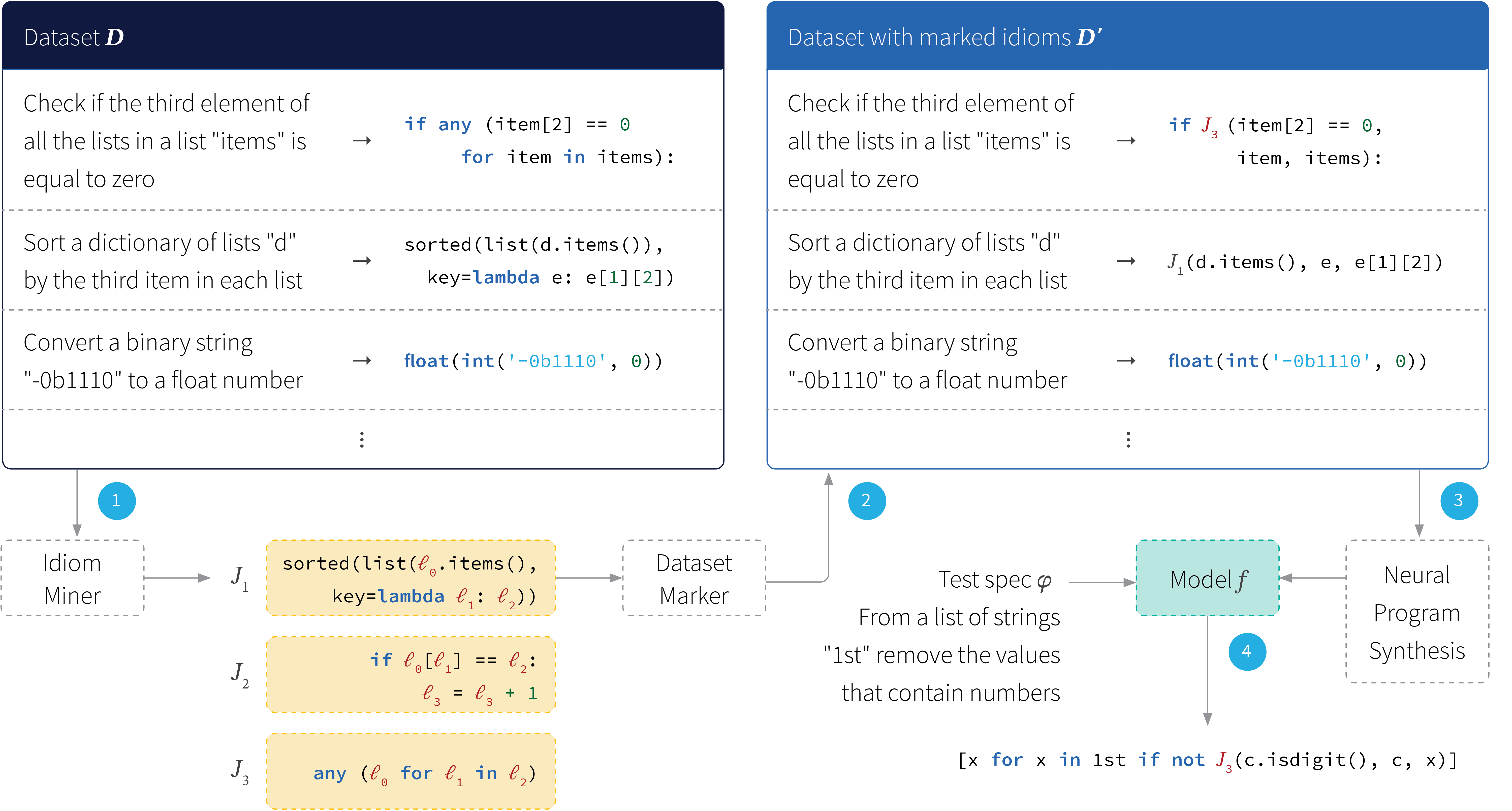
Figure 10. An overview of the `Patois’ program synthesis system. A dataset is mined for code idioms. These are then marked in a second dataset that will be trained for program synthesis. The decoder of this system has the option of outputting the mined code idioms as well as the primitive elements of the abstract syntax tree. As such the system reasons about the output at both high and low levels. Adapted from Shin et al. (2019).
The approach taken and how it relates to previous work: The system consists of two steps (figure 10). The goal of the first step is to obtain a set of frequent and useful program fragments. These are referred to as code idioms. Programs can be equivalently expressed as abstract syntax tree (AST). Hence, mining code idioms is treated as a non-parametric problem (Allamanis et al., 2018) and represented as inference over the probabilistic tree substitution grammar (pTSG).
The second step exploits these code idioms to augment the synthesis model. This model consists of a natural language encoder and an AST decoder (Yin and Neubig, 2017). At each step, the AST decoder has three possible actions. The first is to expand production rules defined in the original CFG of the source code language, which expands the sub-trees of the program AST. The second is to generate terminal nodes in the AST, such as reserved keywords and variable names. The third type of action is to expand the commonly used code idioms. They are hence effectively added to the output action space of the decoder at each step of generation. The resulting synthesis model is trained to maximize the log-likelihood of the action sequences that construct the right ASTs of the target programs given their natural language specifications.
Results: The paper presents experimental results on the Hearthstone and Spider datasets (figure 11). The experiment results show a noticeable improvement of the Patois system over the baseline model, which does not take advantage of the mined common code idioms. For a more qualitative analysis, Figure 12 presents few examples of the mined code idioms from the Hearthstone and Spider datasets, which correspond nicely to some of the high-level programming patterns for each language.
| Model | Exact match | Sentence BLEU | Corpus BLEU |
|---|---|---|---|
| Baseline | 0.152 | 0.743 | 0.723 |
| PATOIS | 0.197 | 0.780 | 0.766 |
Figure 11. Results on the Hearthstone dataset.
| def __init__(self) : super().__init__($\ell_0$ : str, $\ell_1$ : int , CHARACTER_CLASS.$\ell_3$ : id, CARD_RARITY.$\ell_4$ : id, $\ell_5^?$ ) | $\ell_0$ : id = copy.copy($\ell_1$ : expr) class $\ell_0$ : id ($\ell_1$ : id) : def __init__(self): | SELECT COUNT ( $\ell_0$ : col ), $\ell_1^*$ WHERE $\ell_2^*$ INTERSECT $\ell_4^?$ : sql EXPECT $\ell_5^?$ : sql WHERE $\ell_0$ : col = $terminal |
Figure 12. Examples of code idioms mined from the Hearthstone and Spider datasets. Adapted from Shin et al. (2019).