
The transformer has become the workhorse of modern artificial intelligence. Although it was originally designed for sequence-to-sequence tasks like translation, it has since been adapted to other use cases such as chatbots, image classification, and image generation, and provides a foundation for many other tasks.
Despite these successes, the transformer has a major disadvantage: the computational complexity of inference (i.e, running the network) grows as a function of the input sequence length. This is particularly problematic when it is used to generate new words to extend an existing text sequence; the process gradually slows down as the sequence gets longer. Hence, chatbots can be surprisingly computationally expensive to deploy.
Given that the transformer plays such an important role in AI, it’s reasonable to question whether it can be improved or replaced entirely with a different building block. This blog starts with a brief description of the transformer and explains why inference depends on the sequence length. It then describes a family of methods that aim to make inference more efficient. In particular, we discuss attention-free transformers, RWKV, linear transformers, Performers, and the retentive network.
Transformers
This section briefly describes the properties of a transformer decoder network, so that we can then discuss how they might be improved. Readers who are already familiar with transformer decoder networks may skip this section. For a much more detailed discussion, see our previous series of blogs.

Figure 1. Transformer layer. The transformer layer takes a series of embeddings (here representing words) as input and returns a set of modified embeddings. It first combines these via a self-attention mechanism and then processes each separately using identical fully connected neural networks.
Transformer layer
A transformer decoder network consists of a series of transformer layers. Each transformer layer receives a set of $N$ fixed-length embeddings (stored in the $N$ rows of a matrix $\mathbf{X}\in\mathbb{R}^{N\times D}$) and returns a set of $N$ transformed embeddings of the same size. The embeddings may represent word fragments or parts of an image, depending on the task.
Each transformer layer first combines these embeddings using a dot-product self-attention mechanism and subsequently processes each output embedding separately by passing them through identical fully connected neural networks (Figure 1). In practice, both of these components are wrapped in a residual connection, and layer normalization is applied at each to facilitate training.
The dot product self-attention mechanism $\bf{Sa}[\mathbf{X}]$ first computes three quantities, known as queries, keys, and values:
\begin{eqnarray}
\mathbf{Q} &=& \mathbf{X}\boldsymbol\Omega_{q}\nonumber \\
\mathbf{K} &=& \mathbf{X}\boldsymbol\Omega_{k}\nonumber \\
\mathbf{V} &=& \mathbf{X}\boldsymbol\Omega_{v},\tag{1}
\end{eqnarray}
where the rows of $\mathbf{Q},\mathbf{K}$, and $\mathbf{V}$ contain the queries, keys, and values for each embedding, respectively. The matrices $\boldsymbol\Omega_{q}, \boldsymbol\Omega_{k}$, and $\boldsymbol\Omega_{v}$ are learned parameters. In the simplest form of dot-product attention, the queries, keys, and values are combined as:
\begin{equation}
{\bf{Sa}}[\mathbf{X}] = \bf{Softmax}\left[\mathbf{Q}\mathbf{K}^T\right]\mathbf{V}.
\tag{2}
\end{equation}
This computation can be interpreted as follows. Each output (row) of the self-attention mechanism is a weighted sum of the values, where the weights are determined by the dot product (similarity) between the query associated with that input and all of the keys. The quantity $\mathbf{Q}\mathbf{K}^T\in\mathbb{R}^{N\times N}$ contains these dot products which are passed through a softmax function $\bf{Softmax}[]$ that operates separately on each row of the argument. After this operation, the weights sum to one for each output, and these are considered the attention that each output pays to each input. The quantity $\bf{Softmax}\left[\mathbf{Q}\mathbf{K}^T\right]$ is termed the attention matrix.
The computation can also be written in terms of the individual inputs $\mathbf{X}_{n}$ which form the rows of $\mathbf{X}$:
\begin{equation}
{\bf{Sa}}[\mathbf{X}]_{n} = \frac{\sum_{m=1}^{N} \exp[\mathbf{q}_{n}\mathbf{k}_{m}^T]\mathbf{v}_{m}}{\sum_{m=1}^{N}\exp[\mathbf{q_{n}}\mathbf{k}_{m}^T]},
\tag{3}
\end{equation}
where we have written out the softmax function explicitly and $q_{n}$, $k_{n}$, and $v_{n}$ represent the $n^{th}$ row of the queries, keys, and values matrices, respectively.
In practice, the self-attention mechanism usually includes a scaling factor to ensure that the softmax does not saturate and often incorporates some manipulation of the attention matrix to embed information about position. This is discussed in detail in our previous series of blogs.
Transformer decoder
A transformer decoder consists of a series of transformer layers. Its input is a series of tokens, each of which is mapped to a learned embedding, and its output is a probability distribution over the subsequent token in the sequence (Figure 2). In the context of language tasks, each token represents a word or word fragment, so the transformer decoder returns a distribution over possible next words/word fragments in the sequence. By sampling from this distribution and feeding the extended sequence back into the transformer decoder, it’s possible to continue the sequence indefinitely.

Figure 2. Transformer decoder network. A transformer decoder network consists of a series of transformer layers. It receives the embeddings corresponding to a partial sequence of tokens as input and returns a probability distribution over the subsequent token as output.
The probability distribution over the next token is computed by adding a linear function that projects the last output embedding to the dimension of the vocabulary of possible tokens and passing the result through a softmax function. As described, this network could be trained using ground sequences of text, where we know the next token. However, this is very inefficient; to exploit a sequence containing $N$ tokens (preceded by a special $\textcolor[rgb]{0.45, 0.30, 0.98}{<start>}$ token), we would have to pass each of the $N$ possible partial sequences through the model.
The efficiency can be improved by passing the sequence through just once and predicting the continuation of each partial sequence concurrently. Here, every output embedding is mapped to a probability distribution over the subsequent token (Figure 3). Unfortunately, this scheme is problematic since these subsequent tokens are themselves contained in the input sequence, so the network can ‘cheat’. This difficulty can be resolved by noting that the tokens only interact in the self-attention mechanism. For each output, we set the attention weights so that they are zero for subsequent tokens in the sequence, so cheating is impossible.

Figure 3. Predicting multiple output tokens simultaneously. To improve training efficiency, the decoder network predicts the continuation of every sub-sequence simultaneously. Unfortunately, this introduces the problem that the correct responses form part of the input, so the network can learn to ‘cheat’.
This can be achieved by setting elements of $\mathbf{Q}\mathbf{K}^{T}$ above the diagonal to negative infinity so that they become zero after the softmax function. It can also be expressed in terms of the individual output vectors, which are now calculated as:
\begin{equation}
{\bf{Sa}}[\mathbf{X}]_{n} = \frac{\sum_{m=1}^{n} \exp[\mathbf{q}_{n}\mathbf{k}_{m}^T]\mathbf{v}_{m}}{\sum_{m=1}^{n}\exp[\mathbf{q_{n}}\mathbf{k}_{m}^T]},
\tag{4}
\end{equation}
where the sum is now to $n$ (the current input) rather than $N$ (the total number of inputs) as in equation 3. This is known as masked self-attention (Figure 4).
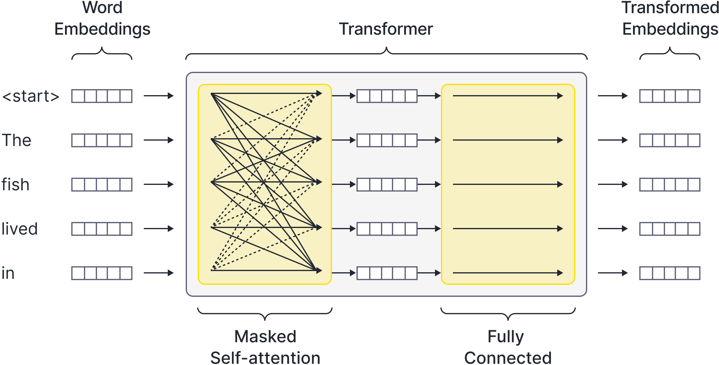
Figure 4. Masked self-attention. To prevent the network cheating, the self-attention mechanism is modified so that the attention paid to subsequent tokens is set to zero and the network cannot ‘look ahead’ to find the true continuation of each sub-sequence. In practice, this means that the dotted connections are removed and only the solid arrows remain.
Problems with transformers
In the previous section, we discussed how training transformer decoders can be sped up by simultaneously processing each partial sequence in parallel (using masked self-attention to avoid cheating). During training, each query interacts with all of the keys that are at the same position or earlier in the sequence. Hence, training naturally has a quadratic dependence on sequence length.
However, it is not possible to perform inference (generate new tokens continuing the sequence) in parallel. We start with a partial sequence and pass this through the transformer decoder. The output from the last token embedding is a probability distribution over possible next tokens. We sample from this (or do something more sophisticated) and then feed the extended sequence back into the model (Figure 5).
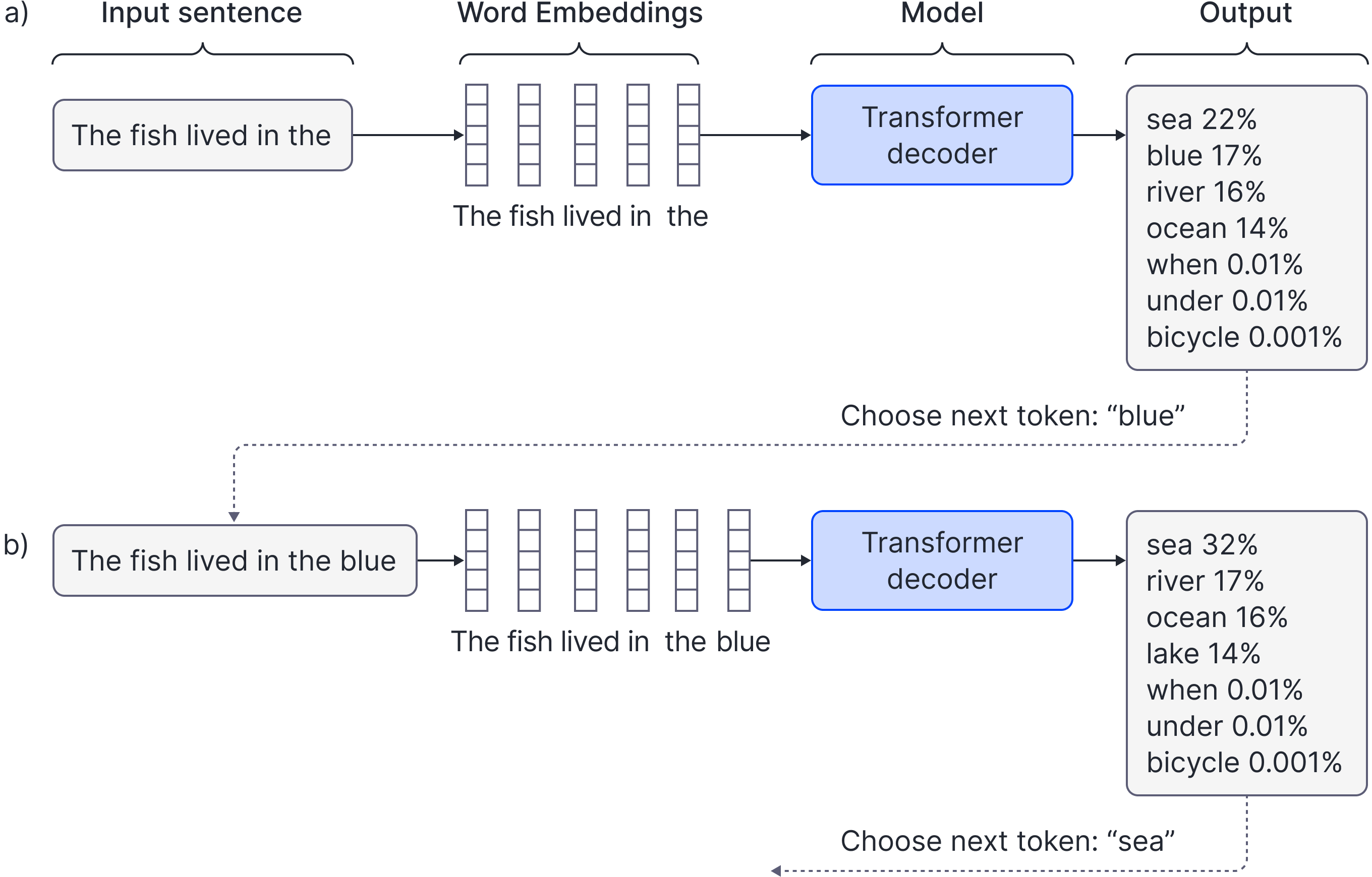
Figure 5. Inference in transformer decoder models. A partial sequence is tokenized, converted to (word) embeddings, and then passed through the decoder network. This creates a probability distribution over the next token, from which we can sample.
It’s worth considering how much computation is required to add a further token to a sequence that already contains $N$ tokens. Considering the computation for just the $N^{th}$ output, we see that $N$ terms must be computed:
\begin{equation}
{\bf{Sa}}[\mathbf{X}]_{N} = \frac{\sum_{m=1}^{N} \exp[\mathbf{q}_{N}\mathbf{k}_{m}^T]\mathbf{v}_{m}}{\sum_{m=1}^{N}\exp[\mathbf{q_{N}}\mathbf{k}_{m}^T]}.
\tag{5}
\end{equation}
It follows that inference gradually slows down as the sequence length $N$ grows longer. In practice, this dependence (plus the quadratic dependence during training) poses bounds on the maximum sequence length that a transformer decoder model can handle. For example, ChatGPT used a context length of only 4096 tokens, and the largest version of GPT4 used a context length of 32,768 tokens. Without further refinements, this means that it isn’t possible to input large bodies of text (e.g, a complete book) and expect the model to cope.
Transformers vs RNNs
It is interesting to compare the computational demands of the transformer with those of the recurrent neural network (RNN). In an RNN, each token is processed in sequence, and each is used to predict a distribution over the next token. At each stage, the RNN outputs a hidden state that is passed forward to the next position and summarizes the history of the sequence. In training, each output is compared to the ground truth next tokens (Figure 6a). In inference, the output distribution is sampled from and the sampled token is fed back into the network at the next position.
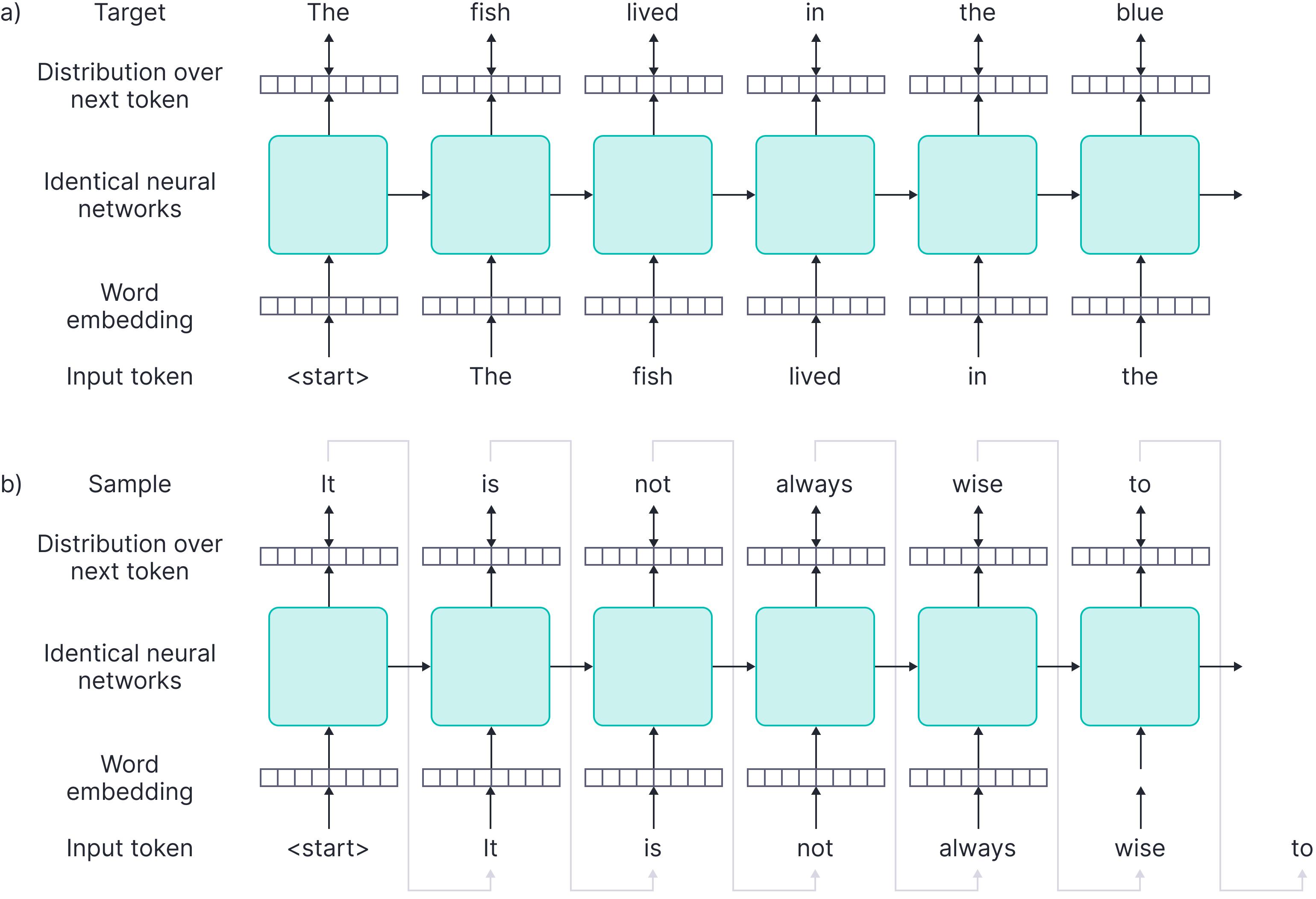
Figure 6. Recurrent neural networks. a) Training. The first $\textcolor[rgb]{0.45, 0.30, 0.98}{<start>}$ token is fed into the a neural network which predicts a distribution over the next token. This is compared to the ground truth target token $\textcolor[rgb]{0.45, 0.30, 0.98}{The}$. The ground truth target token is fed into the identical network at the next position, together with a hidden representation (horizontal arrow) that is also computed at the first position. Hence, training cannot be done in parallel. This contrasts with transformers that process the whole sequence at once. b) Inference. In inference, a new token is sampled at position one based on the network output. This is fed into position two (gray arrows) together with the hidden representation computed at position one. Hence, inference only directly depends on the previous computation and not the entire history and does not grow more demanding as the sequence length increases. This contrasts with transformers, where each subsequent token must attend to ${all}$ the previous tokens and inference slows down as the sequence grows longer.
In contrast to transformers, generating a new token only depends on the new token and the (fixed size) hidden representation passed from the previous position, so inference proceeds at a constant rate and does not slow down as inference proceeds. However, it has the disadvantage that training cannot be done in parallel; each input token must be processed before the next.
Neither the transformer nor the RNN are ideal. An improved model would combine the advantages of both schemes; we would be able to train in parallel but perform inference sequentially without it becoming more costly as the sequence length increases.
Re-thinking the attention matrix
The fundamental problem with dot product attention is that every token interacts with every other before the softmax non-linearity. Hence, we need all of the pre-softmax values to compute the attention that the next token pays to the previous tokens. It follows that if we could redefine the attention computation so that it does not have this property, it might be possible to make inference more efficient.
This section reviews a family of methods that do just this. The attention-free transformer and RWKV both compute an attention value that just depends on the tokens themselves rather than the interaction between tokens. Linear Transformers and Performers both treat the softmax operation as a kernel function and approximate it with a dot product of nonlinear functions of the queries and keys. Finally, the retentive network dispenses with the softmax operation altogether. We now consider these schemes in turn.
Removing token interaction
Each row of the attention matrix indicates how much output $n$ should weight the values from input $m$. In a sentence like The fish lived in the blue sea, these might indicate that the token sea should receive a large contribution from the related word fish and a smaller contribution from the preposition in. Since each token attends to every other, the computation is naturally quadratic (Figure 7a).
Attention-free transformers
Attention-free transformers question whether this interaction is necessary. Rather than computing an attention based on the particular combination of inputs, the attention-free transformer computes an attention value relating embeddings $m$ and $n$ that is based on (i) the embedding $m$ (without considering interactions with the current embedding $n$) and (ii) the positions $(m,n)$ of the two embeddings in the sequence. In a sentence like The fish lived in the blue sea, the attention-free transformer might indicate that the representation of sea should receive a large contribution from the word fish simply because fish is a semantically important word, and not because of any relationship between the two words (Figure 7b). It might also indicate that the representation for sea should receive a large contribution from lived simply because it has learned that the seventh token should pay significant attention to the third token (Figure 7c), regardless of the content.

Figure 7. Removing token interaction. a) Attention matrix for full dot product attention. Every output $n$ depends on every input $m$ at the current or previous position in an arbitrary and content-dependent way. Attention-free transformers use b) a content-based term that depends only on the input and not the interaction with the output term and c) a non-content-based term that just depends on the input and output indices. d) RWKV simplifies this latter term to depend only on the difference $n-m$. There is one learned term $\alpha$ when $n=m$ and an exponential fall-off with the learned rate $\omega$ otherwise.
In mathematical terms, this can be expressed as:
\begin{equation}
\mathbf{x}_{n}^{\prime} = \frac{\sum_{m=1}^{n}\exp[\omega_{mn}]\exp[k_{m}]\mathbf{v}_{m}}{\sum_{m=1}^{n}\exp[\omega_{mn}]\exp[k_{m}]},
\tag{6}
\end{equation}
where $\mathbf{x}’_n$ is the $n^{th}$ output of the transformer, $\mathbf{v}_{m}$ is the value vector computed from the $m^{th}$ input and $k_{m}$ is a scalar value that determines the content-dependent importance of the $m^{th}$ input. This is computed as $k_{m}=\mathbf{x}_{m}\boldsymbol\omega_{k}$ where $\boldsymbol\omega_{k}$ is a learned parameter vector. The terms $\omega_{mn}$ are learned parameters that indicate how important the interaction between positions $m$ and $n$ are regardless of the content. This has roughly the same effect as modifying the attention matrix to embed position (see our previous blog). The pre-softmax attentions are now given by $\exp[\omega_{mn}]\exp[k_{m}]$ and do not require dot-products to compute.
For completeness, we note that the full attention-free transformer also includes a data-dependent gating function that determines the proportion that is contributed to each dimension:
\begin{equation}\label{eq:ti_attention_free}
\mathbf{x}_n^{\prime} = \mbox{sig}[\mathbf{x}_{n}\boldsymbol\Omega_{sig}]\odot\frac{\sum_{m=1}^{n}\exp[\omega_{mn}]\exp[k_{m}]\mathbf{v}_{m}}{\sum_{n=1}^{n}\exp[\omega_{mn}]\exp[k_{m}]}
\tag{7}
\end{equation}
where $\mbox{sig}[\bullet]$ applies the logistical sigmoid function to each dimension, the symbol $\odot$ represents pointwise multiplication and $\boldsymbol\Omega_{sig}$ is learned. This mechanism is not critical to the argument of this blog.
Complexity
The $n^{th}$ output of an attention-free transformer is a weighted sum of $n$ value vectors $\mathbf{v}_{n}\in\mathbb{R}^{D}$, where the weights are the scalars $\exp[\omega_{mn}]\exp[k_{m}]$. In training, the computation is significantly more efficient than for full dot product attention because there is no need to compute $N^2$ dot products of the form $\mathbf{q}_{\bullet}^{T}\mathbf{k}_{\bullet}$. However, the amount of computation to predict the next token still increases with the sequence length due to the sum in Equation 7.
RWKV
The RWKV (receptance, weight, key, value) model uses a related attention scheme that is even simpler. They note that the main contribution of the term $\omega_{mn}$ that indicates how much importance position $n$ should assign to position $m$ (regardless of the content) is to ensure that tokens that are far away from each other interact less. They hence suggest that the terms $\omega_{mn}$ can be replaced by terms that depend only on the distance $d_{mn}$ between the tokens (Figure 7d):
\begin{equation}
\mathbf{x}_{n}^{\prime} = \frac{\sum_{m=1}^{n}\exp[k_{m}]\exp[-d_{mn}]\mathbf{v}_{m}}{\sum_{m=1}^{n}\exp[k_{j}]\exp[-d_{mn}]},
\tag{8}
\end{equation}
where the distance is defined as:
\begin{equation}
d_{mn} = \begin{cases}
(n-m)\omega & \quad n> m\\
\alpha & \quad n= m
\end{cases}.
\tag{9}
\end{equation}
Here, the first case determines the exponential fall-off with distance, controlled by scalar parameter $\omega$, and the second case determines how much the current position contributes to itself.
Note that this attention mechanism is just one part of RWKV, which is a sophisticated architecture that alternates between combining times (as in standard attention) and combining the channels, and also incorporates elements from RNNs. A full description of RWKV is beyond the scope of this article.
Kernelizing the attention matrix
A second approach to making self-attention more efficient to approximate the attention computation using kernel methods. The premise is that self-attention for the $n^{th}$ query can thought of as a special case of the following computation:
\begin{equation}
\mathbf{x}_{n}^{\prime} = \frac{\sum_{m=1}^{n}\mbox{sim}[\mathbf{q}_{n},\mathbf{k}_{m}]\mathbf{v}_{m}}{\sum_{m=1}^{n}\mbox{sim}[\mathbf{q}_{n},\mathbf{k}_{m}]}
\tag{10}
\end{equation}
where $\mbox{sim}[\bullet,\bullet]$ returns a measure of similarity between the two arguments. For dot-product self-attention, this is defined as $\mbox{sim}[\mathbf{q}_{n}, \mathbf{k}_{m}] = \exp[\mathbf{q}_{n}\mathbf{k}_{m}^{T}]$.
Since this similarity is a function of dot products, we can treat it as a kernel function, and as such it can equivalently be written as the dot product of non-linear transformations $\bf{z}[\bullet]$ of the inputs
\begin{equation}
\mbox{sim}[\mathbf{q}_{n}, \mathbf{k}_{m}] = {\bf z}[\mathbf{q}_{n}]{\bf z}[\mathbf{k}_{m}]^{T},
\tag{11}
\end{equation}
which means that the output becomes:
\begin{eqnarray}\label{eq:kernel_rearrange}
\mathbf{x}_{n}^{\prime} &=& \frac{\sum_{m=1}^{n}{\bf z}[\mathbf{q}_{n}]{\bf z}[\mathbf{k}_{m}]^{T}\mathbf{v}_{m}}{\sum_{m=1}^{n}{\bf z}[\mathbf{q}_{n}]{\bf z}[\mathbf{k}_{m}]^{T}}\nonumber \\
&=&\frac{{\bf z}[\mathbf{q}_{n}]\sum_{m=1}^{n}{\bf z}[\mathbf{k}_{m}]^{T}\mathbf{v}_{m}}{{\bf z}[\mathbf{q}_{n}]\sum_{m=1}^{n}{\bf z}[\mathbf{k}_{m}]^{T}},
\tag{12}
\end{eqnarray}
where we have used the associativity property of matrix multiplication between the first and second lines.
If we could find ${\bf z}[\bullet]$ such that ${\bf z}[\mathbf{q}_{i}]{\bf z}[\mathbf{k}_{j}]^{T} = \exp[\mathbf{q}_{i}\mathbf{k}_{j}^{T}]$, then this could be much more efficient because the query and key terms are now decoupled; we only need to compute one dot product between ${\bf z}[\mathbf{q}_{i}]$ and the partial sum $\sum_{m=1}^{n}{\bf z}[\mathbf{k}_{m}]^{T}\mathbf{v}_{m}$ rather than compute dot products between every query and every key. Unfortunately, however, it turns out that although such a non-linear transform ${\bf z}[\bullet]$ does exist, it maps the argument to an infinite dimensional space. From a computational viewpoint, this is not very helpful.
Linear transformers and the performer
There have been two main approaches to resolving this problem. The linear transformer implicitly uses a different measure of similarity ${\bf sim}[\mathbf{a},\mathbf{b}] = {\bf z}[\mathbf{a}]{\bf z}[\mathbf{b}]^{T}$ by defining a function ${\bf z}[\bullet]$ which is more tractable. In particular, it uses ${\bf z}[\mathbf{a}] = {\bf elu}[\mathbf{a}]+1$ where ${\bf elu}[\bullet]$ is the exponential linear unit which is a pointwise non-linearity. In contrast, the performer attempts to approximate the standard dot-product similarity using a finite-dimensional mapping ${\bf z}[\bullet]$. The latter approach is empirically more successful, but still performs worse than the original transformer. However, there are many tricks for training transformers that are targeted at the original softmax function, so it is difficult to draw strong conclusions about performance.
Reformulation as an RNN
We already noted that the decoupling of the query terms from the key terms (which are no longer combined in a softmax function) means that the computational complexity of these kernel-based approaches is lower than for the original dot product attention. In fact, it’s easy to show that these methods can be viewed as a special case of an RNN by rewriting the computation as:
\begin{eqnarray}
\mathbf{x}_{n}^{\prime} &=& \frac{{\bf z}[\mathbf{q}_{n}]\sum_{m=1}^{n}{\bf z}[\mathbf{k}_{m}]^{T}\mathbf{v}_{m}}{{\bf z}[\mathbf{q}_{n}]\sum_{m=1}^{n}{\bf z}[\mathbf{k}_{m}]^{T}} \nonumber \\
&=& \frac{{\bf z}[\mathbf{q}_{n}]\mathbf{A}_{n}}{{\bf z}[\mathbf{q}_{n}]\mathbf{b}_n},
\tag{13}
\end{eqnarray}
where $\mathbf{A}_{n}$ and $\mathbf{b}_{m}$ represent the partial sums in the numerator and denominator respectively. If we initialize $\mathbf{A}_{0}$ and $\mathbf{b}_{0}$ to zero, we can compute all the terms efficiently by iterating:
\begin{eqnarray}
\mathbf{A}_{n}&\leftarrow&\mathbf{A}_{n-1}+ {\bf z}[\mathbf{k}_{n}]^{T}\mathbf{v}_{n}\nonumber \\
\mathbf{b}_{n}&\leftarrow&\mathbf{b}_{n-1}+ {\bf z}[\mathbf{k}_{n}]^{T}\nonumber \\
\mathbf{x}_{n}^{\prime}&\leftarrow& \frac{{\bf z}[\mathbf{q}_{n}]\mathbf{A}_{n}}{{\bf z}[\mathbf{q}_{n}]\mathbf{b}_n}.
\tag{14}
\end{eqnarray}
Viewed in this light, these kernel-based methods have an obvious mapping to RNNs. Each position is processed sequentially, and the quantities $\mathbf{A}_{n}$ and $\mathbf{b}_{n}$ from equation 14 form the hidden representation (Figure 8).
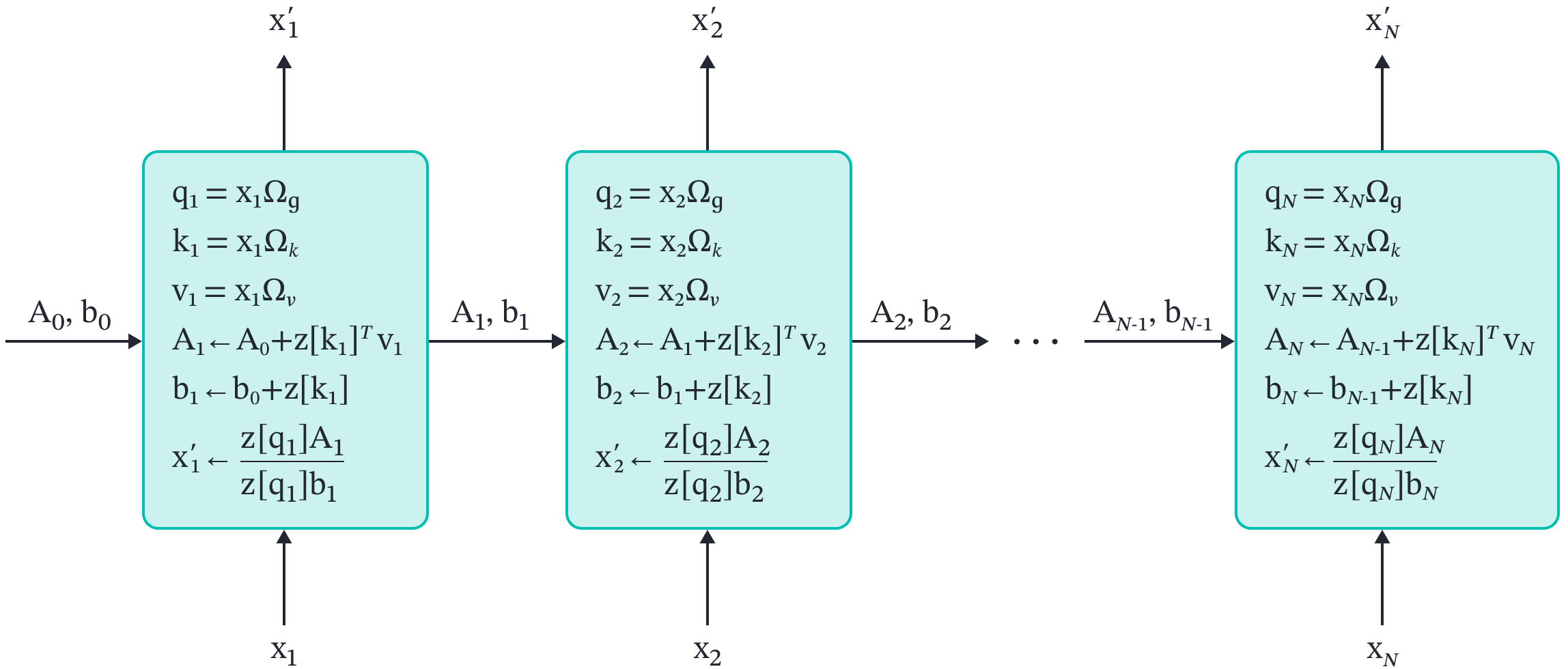
Figure 8. Kernel-based attention as an RNN. The computations for kernelized attention in equation 14 can be viewed as an RNN, in which the hidden state consists of the partial sums $\mathbf{A}_{n}$ and $\mathbf{b}_{n}$. The amount of computation to predict a new output is constant, regardless of the length of the sequence.
Hence, these kernelized attention methods combine the advantages of transformers and RNNs. Like transformers, they can be trained in parallel using all of the terms in the input sequence. Like RNNs, the inference can proceed one term at a time, with a constant cost, so the computation does not increase with the sequence length. Unfortunately, however, they have not yet been shown to be empirically as successful as the original transformer.
Retentive network
The retentive network is a very recent network architecture that also simplifies dot product attention so that it can be represented as an RNN. Again, inference does not become more expensive as the sequence length increases. Unlike the other architectures discussed so far, it appears to scale as well as the original transformer, and the authors claim that it performs better (Figure 9). Note, however, that at the time of writing, this work is still under review, so the reader should retain some skepticism about these claims.

Figure 9. Retentive network vs. transformer performance. a) With sufficient parameters, a retentive network models language better than an equivalent transformer network. It also b) uses less GPU memory, c) has higher throughput, and d) has less latency. See $\href{https://arxiv.org/abs/2307.08621}{\color{blue} \mbox{Sun et al. (2023)}}$ for more details.
The main idea of the retentive network is to remove the softmax function, so the attention matrix is now computed as:
\begin{equation}
\mathbf{X}’ = (\mathbf{Q}\mathbf{K}^{T}\odot{\mathbf{M}})\mathbf{V},
\tag{15}
\end{equation}
where as usual, the rows of the matrices $\mathbf{Q}, \mathbf{K}$, and $\mathbf{V}$ contain the queries, keys, and values, respectively. The matrix $\mathbf{M}$ is a matrix containing ones in lower-triangular positions and zeros elsewhere and the operator $\odot$ represents pointwise multiplication. This enforces the masking so that the network cannot cheat during training.
As usual, the individual outputs $\mathbf{x}’$ can be written as a sum:
\begin{eqnarray}
\mathbf{x}_n’ &=& \sum_{m=1}^{n}\mathbf{q}_{n}\mathbf{k}_{m}^{T}\mathbf{v}_m\tag{16} \\
&=& \mathbf{q}_{n}\sum_{m=1}^{n}\mathbf{k}_{m}^{T}\mathbf{v}_m,
\tag{17}
\end{eqnarray}
where in the second line we have used the associative property of matrix multiplication. As for the kernel-based methods, the queries and keys are decoupled. Comparing this to the kernel-based formulation in equation 12, we see that it is exactly the same, except that we no longer pass the queries and kernels through the function ${\bf z}[\bullet]$ (or equivalently, that function is the identity) and we no longer normalize.
The retentive network also incorporates two mechanisms for indicating relative position information. First, the queries and keys are computed as:
\begin{eqnarray}
\mathbf{q}_{n} &=& \exp[i\theta n] \cdot\mathbf{x}_{n}\boldsymbol\Omega_{q}\tag{18}\\
\mathbf{k}_{m} &=& \exp[-i\theta m]\cdot\mathbf{x}_{m}\boldsymbol\Omega_{k},
\tag{19}
\end{eqnarray}
so every element of the query matrix is rotated by $n\theta$ in the complex plane, and every element of the key matrix is rotated by $m\theta$ where $\theta$ is a learned parameter. The result of this is that when $n=m$, the dot product is computed as usual. As $|n-m|$ departs from zero, there is a progressive increase in the angle in the dot product, which decreases (as long as $|n-m|\theta$ is less than $\pi/2$ radians or 90 degrees); the dot product is increasingly down-weighted as the two positions become more distant. This is a version of the rotary position embedding.
The second mechanism to indicate relative position information is to add another term
\begin{eqnarray}
\mathbf{X}_n’ &=& \sum_{m=1}^{n}\gamma^{n-m}\cdot \mathbf{q}_{n}\mathbf{k}_{m}^{T}\mathbf{v}_m\tag{20} \\
&=& \gamma^{n}\cdot \mathbf{q}_{n}\sum_{m=1}^{n}\gamma^{-m}\cdot \mathbf{k}_{m}^{T}\mathbf{v}_m,
\tag{21}
\end{eqnarray}
where $\gamma\in[0,1]$ is a learned constant. Once more, this has the effect of down-weighting contributions as the distance $|n-m|$ (which is always non-negative) increases.
Reformulation as an RNN
Similarly to the kernel-based methods, the retentive network can be reformulated as an RNN by computing a partial sum $a_{n}$ and adding a term every term at every step (Figure 10):
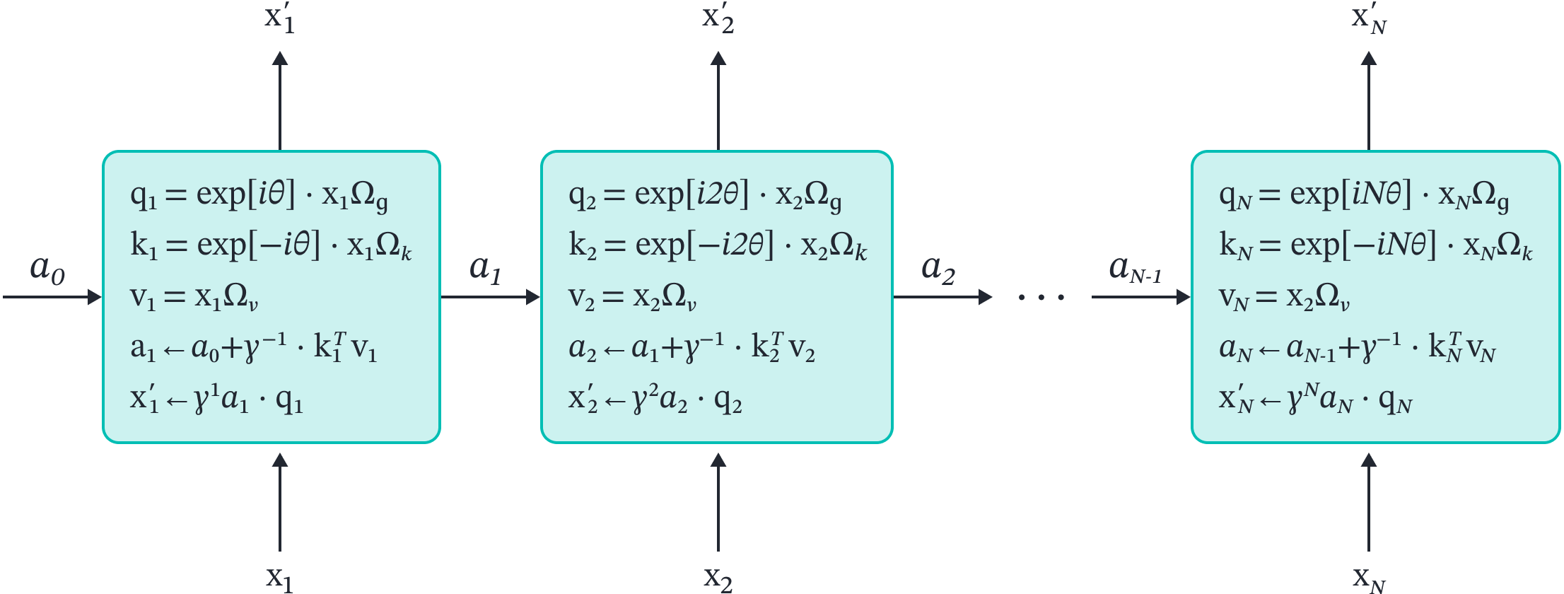
Figure 10. Retentive network as an RNN. The computations for the retentive network in equation 22 can be viewed as an RNN, in which the hidden state consists of the partial sum $a_{n}$. The amount of computation to predict a new output is constant, regardless of the length of the sequence.
\begin{eqnarray}\label{eq:retentive_rnn}
a_n &\leftarrow&a_{n-1}+ \gamma^{-n}\cdot \mathbf{k}_{n}^{T}\mathbf{v}_{n}\nonumber \\
\mathbf{x}_{n}^{\prime}&=& \gamma^{n}a_{n}\cdot\mathbf{q}_{n} .
\tag{22}
\end{eqnarray}
Once again, there is a constant amount of computation to predict each output in inference, so the generation of sequences does not slow down as the sequence gets longer.
Retentive network details
To make the performance competitive with a transformer network, the retentive network makes several other changes:
- The LayerNorm operations are placed before the retentive network and the fully connected networks but within the residual connection. In fact, this is common in modern implementations of the transformer.
- Each attention uses multiple heads where each head has a different scale factor $\gamma$. Hence, each considers integrating information over different scales. This is termed multi-scale retention.
- Group normalization is applied to the output of the heads before recombination. This may help make the system more numerically stable in the absence of the usual normalization in the softmax function.
- Three methods are used in combination to normalize the outputs of the heads before they are passed into the group normalization operation. This normalization does not affect the final output but ensures that the forward and backward passes are numerically stable.
Conclusion
This blog has reviewed various attempts to simplify the computation of the attention matrix so that inference does not become slower with sequence length. We reviewed attention-free transformers and RWKV, which both remove the quadratic dependence by removing the content-dependent interaction. This reduces training computation, but inference still grows with sequence length. Kernel-based methods such as linear attention and the performer approximate or replace the softmax function with an inner product between non-linear functions of the queries and keys. These can be shown to take the form of an RNN, so computation does not grow with sequence length in inference. However, their performance is not currently state-of-the-art.
At the time of writing, the (not yet reviewed) retentive network represents the best hope for replacing the transformer. The core attention matrix is computed by simply removing the softmax function from the original formulation. This allows us to train in parallel but to treat the system as an RNN during inference; hence computation in inference does not increase with sequence length. When various tricks for encoding relative position, processing multiple scales, and normalizing the representation are added, this network appears to be as good as or better than the original transformer.