Introduction
[Get the code Bitbucket – Framework Eval]
Until now, the Machine Learning (ML) frameworks we’ve used at RBC Borealis have varied according to individual preference. But as our applied team grows, we’re finding that a preference-based system has certain shortcomings that have led to inefficiencies and delays in our research projects. As a result, we identified two main arguments in favour of standardizing a single framework for the lab.
1. Lack of reusability
It has been our experience that independent frameworks do not often “play well” together. For example, a TensorFlow-based model applied to one research project would have to be rewritten in PyTorch for another project. When teams had to adapt code in order to fit it to the new framework, it wasted time and slowed their pace. Additionally, the lack of framework consistency meant it was harder for researchers to find someone who could help them out in a pinch if they faced any of the complexities that can arise when debugging machine learning models.
2. Depth vs. breadth
The more exposure we have to the kinds of errors that can emerge from one framework, the more useful we can be to the rest of the team than only having a bit of exposure to a few problems across multiple frameworks. Better to have strong, collective wisdom on one framework versus a shallow knowledge base of many.
Natural selection
But first, we needed to compare frameworks in order to test which one was best for our purposes. Typically, our projects start with vague specifications on what needs to be done, followed by a heavy research component where the goal is to iterate quickly and converge on the best model architecture. So our primary criteria was in selecting a framework based on features that support rapid iteration.
And since speed is of the essence, we need to debug code without too many complications. A community support that allows us to learn the framework quickly and get exposure to the different kind of problems we may face is crucial. It’s also important to be able to modify or extend the framework; for example, implementing new types of LSTM or RNN cells.
For this reason, we decided to run this experiment using PyTorch and MXNet. We chose these two platforms because they are both known to be quick and efficient, while at the same time providing dynamic computational graphs (for further explanation on dynamic computational graphs please see the “Discussion” section below), which allow for fairly easy code debugging.
Finally, they both present their individual strengths: PyTorch is very widely used in the research community which means we can pull from the large pool of code snippets already in circulation. MXNet, on the other hand, is really fast and we wanted to compare its speed to PyTorch.
Note that we left out TensorFlow in our comparison. Although TensorFlow recently came out with Eager Execution, an imperative, define-by-run platform that should make debugging easier, it’s still relatively new.
Infrastructure
For ease of reproducibility, we ran our experiments on an EC2 instance with the following properties:
Instance details
| Spec | Value |
|---|---|
| AMI Id | ami-0a9fac70 |
| EC2 instance | p3.2xlarge |
| GPU Type | Tesla V100 |
| Num GPUs | 1 |
| PyTorch environment | pytorch_p36 |
| MXNet environment | mxnet_p36 |
Software details
The table below contains details of the software in the aforementioned AMI in case it gets updated.
| Spec | Value |
|---|---|
| OS | Ubuntu 16.04 |
| Python | 3.6.3 |
| PyTorch | 0.3.0.post4 |
| MXNet | 1.0.0 |
| CUDA | 9.0.176 |
| CuDNN | 7.0.0.3 |
| NVidia driver | 384.81 |
Data and Model
The implementation is for a binary sentiment classifier using the IMDB dataset with a 50-50 train-test split. There are 50,000 sentences in total with labels being 1 or 0 for positive or negative classes respectively. The data was downloaded via Keras with a vocabulary size of 5000 and a padded sequence length of 500.
An embedding layer produces high-dimensional continuous representations for words in each sentence in the dataset, and a LSTM layer uses these sequences to additionally learn from the context before a word. A fully connected layer decodes the LSTM output, followed by a softmax to give class probabilities. Cross entropy loss is used as the objective function along with Adam as the optimizer.
Experiments
I ran experiments to investigate how computational performance is impacted by varying:
- the number of workers used in data loading
- batch size
- by returning sparse gradients from the embedding layer (PyTorch only)
Performance is measured in terms of runtime for the training component per epoch. The reported time is the average runtime in seconds as measured by python’s `time` library across 20 epochs rounded to 2 decimal places.
I chose to leave out the first epoch in the average time calculations for both frameworks because the compute times fluctuate between subsequent runs. On running the script for the first time on EC2 instances, the first epoch takes anywhere from 300-900% longer (likely due to EBS volume initialization after launching the instance, where the AMI is synced from S3). On subsequent runs the first epoch takes 30-50% longer than other epochs (depending on run parameters).
In some cases it was useful to ballpark the CPU and GPU utilization. CPU utilization was found using the ‘top’ tool on Linux, and GPU utilization was estimated by watching output from ‘nvidia-smi’ and taking the mode of the observed samples. While these are not accurate metrics the relative changes can be useful to know.
Using Sparse Gradients in PyTorch
One suggestion by the PyTorch team was to set ‘sparse=True’ in the embedding layer, which returns sparse gradients instead of dense ones. Since MXNet’s Gluon API does not yet support sparse gradient optimizations (this should be implemented soon), a fair comparison between the two frameworks isn’t possible at the moment. However, we can provide results for PyTorch using both dense (sparse=False) and sparse (sparse=True) gradients to show possible performance improvements.
Results and Analysis
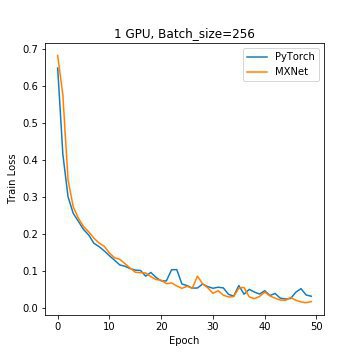
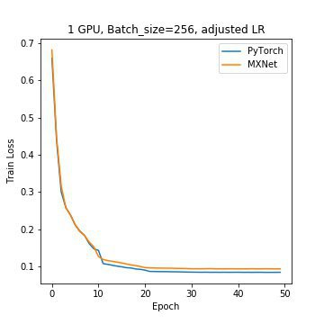
We looked at the training loss curve when running the model with a batch size of 256 and no data workers and noted a significant oscillation in the training loss after about 17 epochs. This made it difficult to draw conclusions about which framework trains better. After adding a factor learning schedule that decays the learning rate by 10% every 10 epochs, we got the results in Figure 2.

Figure 1: Convergence curve for both frameworks with no learning rate scheduled
As you can see, the loss curve is much smoother now and shows that PyTorch trains slightly better than MXNet.

Figure 2: Convergence curve for both frameworks after applying a factored learning schedule
The following tables give average times per epoch across different batch sizes for PyTorch (using dense and sparse gradients) and MXNet (using dense gradients only) with 0, 1, 2 and 4 data loading workers.
Without any workers, Pytorch is about 10% faster than MXNet. CPU utilization (multi-CPU) was higher for MXNet than PyTorch (~120% vs ~100%), and Pytorch had better overall GPU utilization (77% vs 65%). From this observation, one explanation for the higher compute times without any workers could be that MXNet’s main process alone cannot transform and load data quickly enough into the data queue, leaving the GPU under-utilized. PyTorch suffers from this limitation too but not to the extent that it affects MXNet, as demonstrated by better GPU utilization.
Adding a worker improves GPU utilization for both frameworks (80-90% for both). It’s interesting to note that varying the number of workers impacts MXNet more dramatically than PyTorch; increasing the number of workers from 0 to 4 benefits MXNet by up to 130% across different batch sizes, but only benefits PyTorch by up to 5%.
Using sparse gradients with PyTorch improves performance by 20-60%, depending on batch size.
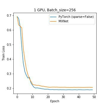
In this particular benchmark setting, the optimal performance for both frameworks comes from a batch size of 1024. Increasing the number of workers from 1 to 2 improves MXNet’s performance by 51.6%, but does not noticeably impact PyTorch. Further increasing the number of workers does not benefit either framework, likely because for this benchmark two workers are sufficient to load the data queues and prevent GPU starvation. With optimal parameters for both frameworks, MXNet is twice as fast as PyTorch using dense gradients, and 20% faster when Pytorch uses sparse gradients. Figure 3 shows the convergence rate for both frameworks and indicates that PyTorch trains better.

Figure 3: Convergence curves at batch-size=1024, num_workers=2
Developing in PyTorch vs MXNet
Static vs Dynamic Graphs
With MXNet, computational graphs can be defined both imperatively (dynamically) with the Gluon API, or declaratively (statically) using the Symbol API, while PyTorch only declares graphs dynamically. If you’re not familiar with these terms, we found this page to be a good resource. Briefly, imperative programming allows for easier debugging since values “stick around”. The advantage is that we can inspect the program state retrospectively at the expense of taking up more memory and computational resources. Declarative programs can optimize both memory and computational requirements, but are tricky to debug. With the Gluon API, programs can be written imperatively and then “hybridized” (i.e., compiled to a static computational graph) at deployment time.
We haven’t hybridized the MXNet implementation because gluon.rnn.LSTM does not support hybridization. We reached out to the MXNet team and the explanation they gave is that gluon.rnn.LSTM already uses a fused RNN implementation, which is as efficient as one can get on a GPU. The recommended usage for hybridization, in this case, is to separate the architecture into pre-LSTM and post-LSTM hybrid blocks and tie all three into a simple block.
Community Support
We found it easier to debug with PyTorch than with MXNet. Standard error output from PyTorch almost always pointed us in the right direction and, in cases where the error messages were vague, the answer was already on StackOverflow or the PyTorch forums. We found error messages from the Gluon API to be less accessible, and the community support just isn’t as good as PyTorch yet.
PyTorch is far more widely adopted in the research community to date, which naturally results in a higher volume of community-contributed solutions to problems that other people would come across. For the same reason, there are also a lot more community-driven implementations that can be reused in your code compared to MXNet.
Documentation
PyTorch’s documentation reads like any good API, with a focus on being comprehensive and providing plenty of examples. The folks at MXNet have additionally tried to teachmachine learning via their Gluon API documentation, which is a useful hands-on resource for someone trying to catch up quickly.
While they’re both well documented frameworks, MXNet’s teaching API is really useful for people just starting out in the field.
Using ONNX to move between frameworks
Open Neural Network Exchange(ONNX) is an open-source format for AI models. Most major frameworks either support or will support importing and exporting models to the ONNX format, potentially allowing us to leverage capabilities of multiple frameworks. One outcome of ONNX could be to use PyTorch when we need to move quickly in our research, then switch over to MXNet once performance becomes the dominant factor.
Conclusion
In summary, we found that MXNet is twice as fast as PyTorch for this benchmark when using a batch size of 1024 and 2 workers. With a model using an embedding layer in PyTorch, we arrived at a performance boost of 20-to-60% by setting sparse=True.
Given its widespread community support, simple API, and intuitive error messages, we can see PyTorch being used in Applied Research at RBC Borealis while we’re in the process of debugging a model. Once we have the pipeline figured out, it makes more sense for us to switch to MXNet and leverage its faster performance, possibly by exporting the PyTorch model to ONNX and importing to MXNet.
Acknowledgements
I’d like to thank Joey Bose, JinSung Kang, Yevgeniy Vahlis and the RBC Borealis team for their help with this post. I’d also like to thank Sina Afrooze (MXNet team) and the PyTorch team for their feedback on the MXNet and PyTorch implementations, respectively.
Edit 1: Thanks to Soumith from the PyTorch team for pointing out that setting “sparse=True” does not change the Embedding layer to use sparse embeddings, what’s sparse is the gradients returned. I added a note to clarify this in the Experiments section and updated the tables accordingly.