
Foundation models are large-scale AI models that are pre-trained on a vast dataset and enable seamless generalization across tasks. As one of Canada’s largest banks based on market capitalization, RBC has access to significant amounts of data and compute. This plays a critical role in our ability to create high value and differentiating models like ATOM, RBC’s foundation model for financial services. We trained ATOM on large-scale financial time-series datasets comprising billions of client interactions such as payment data, stock market trades, and loyalty rewards, supercharging its decisioning power with the sprawling and specialized knowledge domain that is Financial Services.
Training a foundation model on tens of billions of data points is computationally expensive and time-intensive; even small improvements to training efficiency dramatically boost iteration speed and therefore delivery. In the course of building ATOM, we encountered a common difficulty in building foundation models: the fastest way to process data is to avoid reading from disk and process in-memory, but memory is finite and therefore data pipelines don’t scale.
In this blog, we discuss how we addressed the bottleneck of doing in-memory processing during training by using memory mapping with the Arrow format, unlocking considerable reduction in memory requirements compared to our original solution.
Our data storage and retrieval approach
Our data storage system consists of two sets of tables. The first, the dimensions table, contains identification details for each time series, indexed by sample_id. It also includes start and end indices that define the range of events corresponding to each time series in the second table, the time series table. The time series table stores the actual event data, grouped and sorted by sample_id. We use the indices from the dimensions table to efficiently locate specific time series data. Since each sample can contain thousands of time-series events, the time series table is significantly larger than the dimensions table.
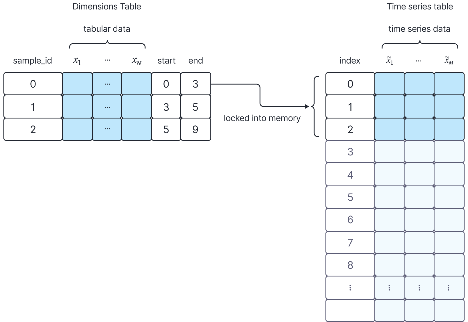
Figure 1: we select the time series belonging to sample i=1 in the dimensions table from the time series table. This is done using the pre-computed start and end indices in the dimensions table.
To retrieve a given sample during training, we select the i-th row from the dimensions table, and using the start and end indices, slice the corresponding time-series information. In our original design, we loaded both tables into memory, but this approach soon became untenable because it failed to scale as the tables grew in size. At one point, we were consuming 500GB of memory at a time for training alone.
Ultimately, we want to design a scalable solution that allows us to do blazing fast processing. As we know, in-memory processing offers that, however memory is finite and can’t keep up with data growth. We need a way to use available memory efficiently by loading only the necessary information. An important step towards that goal is to leverage data storage formats that allow for reading larger-than-memory datasets and fast random access. Hence, in order to achieve our vision of training models on large datasets, we need a way for efficient data loading, and choose the right file format that enables it.
Choosing the right file format
The choice of storage format for time series datasets is an important piece to formulate a complete solution. For us, we want to achieve the following:
- Read larger than memory datasets
- Fast random access given an identifier
- Positive development and user experience
Possible Solutions
After careful consideration, we narrowed down the list of possible file formats to just 3: Parquet, Memory-mapped Numpy arrays, and Apache Arrow. To select a winner, we benchmarked each format to learn how efficiently each format could fetch a target set of time-series records given a random batch of identifiers.
Arrow defines two binary representations: the Arrow Streaming Format and the Arrow IPC File (or Random Access) Format.
- Arrow Streaming Format is optimized for real-time data transfer and lacks random access, and must be processed sequentially
- Arrow IPC File Format (Feather) supports random access with a footer with necessary metadata for efficient navigation
- Both formats use Arrow’s efficient memory model but are designed for different use cases: streaming for real-time data and IPC file format for static, persistent storage
To read large Arrow datasets more efficiently from disk, we use memory mapping. This approach enables direct access to data with lazy loading, allowing for random access without needing to load the entire file into memory upfront.
Benchmarking
Dimensions for evaluation: time and memory
- We fix the following:
- number of rows in the raw time series data to 400 million
- 10 columns consisting of mix of data types, including string, booleans, floats and ints
- batch size (= 512) representing identifiers for random retrieval for our data loader
- amount of memory available to process to 8G
- number of rows in the raw time series data to 400 million
- Once we extract the rows corresponding to a client, we transfer them from CPU to the GPU
- We also repeated the experiments for 1 epoch (= 330 batches)
We measure the time for reading the file and retrieving one batch.
| File Format | File read time (s) | Time to retrieve one batch (s) | Speedup relative to parquet | Notes |
|---|---|---|---|---|
| Parquet | 0 | 160 | – – | – We used DuckDB to retrieve the data from the parquet file – Parquet files do not allow direct memory-mapped I/O due to their compressed nature – Focus is space-efficient I/O |
| Numpy Memory Mapped Array(s) | 0.013 | 4 | 40x | – Represent each column in time series data as one memory-mapped array – Not easy to use as we need to implement custom data structure to hold time series data |
| Arrow IPC (memory mapped) | 0.26 | 4 | 40x | – We used a wrapper on top of PyArrow to retrieve the data – Arrow is not recommended for long-term storage as its size could be up to 10x of the equivalent parquet file We use Arrow datasets as an intermediate step, to train our models and do inference, however we choose to continue to store our raw time series data in parquet format |
The memory mapped arrow IPC data format is best suited for our needs because of the following:
- Ability to read larger than memory datasets
- In our benchmarking, we can verify our understanding of memory mapping by restricting the allocated memory to the process
- Fast random access
- Supports “slicing” of data with random access
- Very useful with memory maps
- Positive development and user experience
- Apache arrow has strong open-source community support
- Large investments being made by the wider community to expand this ecosystem
Note that the file read time is slightly slower for Arrow, compared with Numpy in the above table. We consider this acceptable given our primary focus is on the memory and time to slice data.
As we learned that Arrow and memory mapping work well together, let us dive deeper into how memory mapping can specifically help us in data loading as well as any caveats associated with it.
Memory mapping to reduce memory usage
Memory mapping maps a file to a region of the virtual memory available to the process, even if the contents are too big to fit into your physical memory. This allows us to lazily load parts of time series data we need, without having to hold all data in memory.
In order to ensure low memory usage in our solution, we memory map the file containing time series information before reading them and building a PyArrow Table. Because of the mapping we build between dimensions and time series information, constructing this in memory representation is fast and resource efficient for us – given an identifier, we can slice the time series information from multiple sources as we know the range of rows that belong to our identifier. As our time series data is sorted, during model training we can sequentially provide the identifier(s) and request time series information for them, which helps to avoid the overhead associated with page faults by keeping “likely to be accessed” memory locations together.
Our prior approach is shown on the left. We loaded the whole time-series into memory, which is very memory intensive, and select slices from it using the indexing approach mentioned in the previous section.
In our new approach, we lazily load the requested rows into memory.
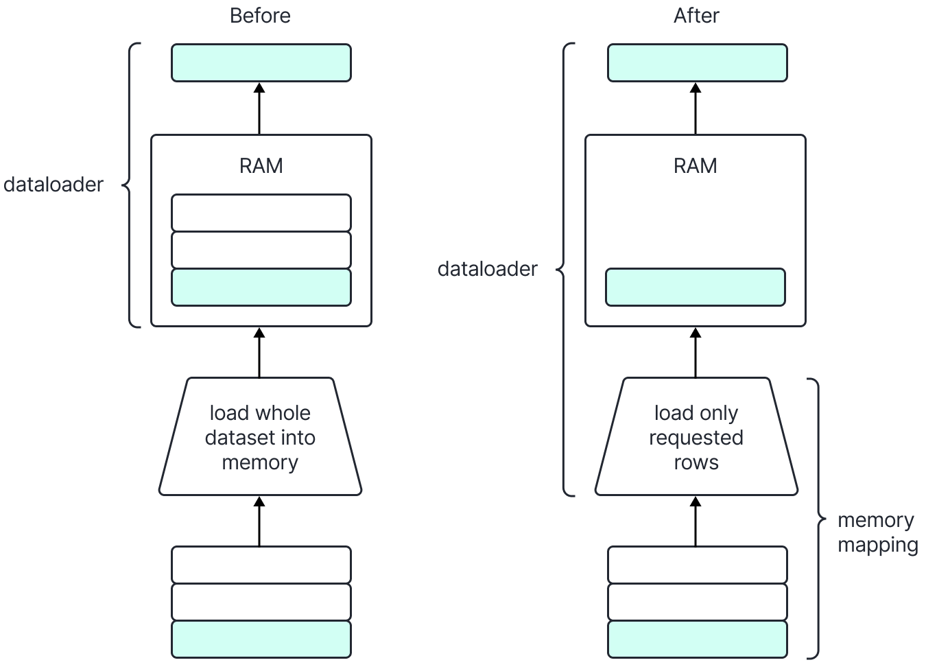
Figure 2: with memory mapping, we only load requested rows into memory when loading data. This reduces our memory usage.
During training, we are interested in retrieving all the time series that are linked to an identifier. This memory mapped solution offers a scalable way allowing us to load only requested data by just slicing our memory mapped representation, without increasing our memory requirements. As seen in the image above, the dataset creator will memory map the Arrow file containing time series data and only load the rows corresponding to the requested identifier in physical memory. This operations helps us scale our training by removing the bottleneck of otherwise holding all time series data in memory, or paying the I/O cost of querying it from a database. This approach decreases our memory requirements by up to 90%.
Memory Mapping is not a silver bullet
Memory mapping however, is not a silver bullet and there are some caveats to keep in mind while using it. For instance,
- No major performance improvements from memory mapping when there isn’t enough physical memory in the system, allowing the OS to compensate by switching to a slower physical storage such as SSD. (source)
- We observed simultaneous read to memory-mapped file to be slow, but not a huge bottleneck.
- In our benchmarking, memory requirements grew sub linearly with file size. For example, if the memory required to process a file of size X was 20G, then memory required to process file of size 5X was 40G.
Getting started with Arrow files is easy
If you’re thinking of getting started with using memory mapped arrow files, it’s easy!
If your data lives as a parquet file, you will want to first convert it to an arrow file to take advantage of memory mapping.
You can use the code below to write the table to disk as an Arrow IPC file. Alternatively, you can do the same operation using DuckDB.
import pyarrow as pa
import pyarrow.parquet as pq

reader = pq.ParquetFile("my_table.parquet")

with pa.ipc.new_file("my_table.arrow", schema=reader.schema_arrow) as writer:
    for batch in reader.iter_batches():
        writer.write(batch)
Then you can read back the same file in a memory-mapped way using the code below:
with pa.memory_map("my_table.arrow", "r") as source:
    table = pa.ipc.open_file(source).read_all()
Conclusion
Introducing Arrow-based Memory-Mapping cuts ATOM’s memory footprint by a whole order of magnitude, down from 500GB to 50GB. While we’ve only tested on time series data so far, our techniques can transfer to any data stored in tabular form. This work has broad implications for organizations having limited computational resources, but wanting to train and quickly iterate on their own models with massive datasets!
Future Work
During our benchmarking, we also experimented with the Apache Feather (V2) format which in itself is based on the Arrow IPC format. We were surprised to see that using the Feather format does not offer the same benefits as operating on the IPC format directly. Under the benchmarking conditions, we found reading Feather files using PyArrow’s API to be quite slow and memory intensive. We will look to dive deeper into this in the future.
We also explored HuggingFace datasets as an interface to use memory mapping with Arrow format, however we decided to implement a custom solution for the kind of time series data we have, allowing us more control over the abstraction. This was beneficial for us as we could couple the designs for the data storage and retrieval mechanisms. Moreover, similar to the case with Feather files, we found reading and retrieval from Arrow files with HuggingFace a lot slower than we anticipated, compared to using the Arrow IPC’s open_file API.
In the future, we would love to revisit our design and see if we can implement it with HF datasets, or use Feather format.
Further details about ATOM can be found here, including a list of our research publications in this space.
Acknowledgements
We would like to thank Kevin Wilson, Jawad Ateeq, Qiang Zhang, Melissa Stabner, and Joelle Savard for their help with reviewing, editing, and refining this blog post.
Want to learn more about ATOM?
RBC Borealis is building ATOM (Asynchronous Temporal Model), a foundation model for financial services.
Explore our work