The transformer has enabled the development of modern language models such as GPT3. At a high level, it is just a network that allows non-linear transformations to be applied to sets of multi-dimensional embeddings. In NLP, these embeddings represent words, but the same ideas have been used to process image patches, protein sequences, graphs, database schema, speech, and time series.
Each of this series of three blogs focuses on different aspects of the transformer. In Part I, we introduce self-attention, which is the core mechanism that underpins the transformer architecture. We then describe transformers themselves and how they can be used as encoders, decoders, or encoder-decoders using well-known examples such as BERT and GPT3. This discussion will be suitable for someone who knows machine learning, but who is not familiar with the transformer.
Part II considers how to adapt the transformer to cope with longer sequences, different methods for encoding the positions of elements in the sequence, and other modifications to the basic architecture. We also discuss the relationship between the transformer and other models. This will be suitable for a reader who knows the basics about transformers and wants to learn more.
Transformer models are difficult to train from scratch in practice. Part III details the tricks that are required to ensure that training does not fail. We conclude with a discussion of our recent work on how to modify the training procedure to fine-tune deep transformers when only sparse training data is available. This discussion will be suitable for practitioners who want to learn more about how to work effectively with transformers.
Motivation
To motivate the transformer, consider the following passage:
The restaurant refused to serve me a ham sandwich, because it only cooks vegetarian food. In the end, they just gave me two slices of bread. Their ambience was just as good as the food and service.
We would like to build a network that can process this passage into a representation that is suitable for downstream tasks. For example, we might want to classify the review as positive or negative, or answer questions such as “Does the restaurant serve steak?”. Two problems immediately present themselves:
First, the input representation will be large. Typically, we might describe each of the 37 words with an embedding vector of length 1024 and so the network input will be of length $37 *1024 = 37888$ even for this small passage. A more realistically sized input might have hundreds or even thousands of words. It’s not clear that a standard fully-connected network would be practical here; it would need a very large number of parameters, and it’s not obvious how to adapt such a network to inputs containing different numbers of words. This suggests the need for some kind of parameter sharing that is analogous to the use of convolutions in image processing.
Second, language is fundamentally ambiguous; it is not clear from the syntax alone that the pronoun it refers to the restaurant and not the ham sandwich. To fully understand the text, the word it should somehow be connected to the word restaurant. In the parlance of transformers, the former word should pay attention to the latter. This implies that there must be connections between the words, and that the strength of these connections will depend on the words themselves. Moreover, these connections need to extend across large spans of the text; the word their in the last sentence also refers to the restaurant.
In conclusion, we have argued that a model that can process real world text (i) will use parameter sharing so that it can cope with long input passages of differing lengths, and (ii) will contain connections between word representations that depend on the words themselves. The transformer acquires both of these properties by using dot-product self-attention.
Dot-product self-attention
A standard neural network layer $\bf nn[\bullet]$, takes a $D\times 1$ input $\mathbf{x}$, applies a linear transformation followed by a static non-linearity like a rectified linear unit (ReLU)
\begin{equation} \bf nn[\mathbf{x}] = \bf ReLU[\boldsymbol\Phi\tilde{\mathbf{x}}], \tag{1}\end{equation}
to return a modified output vector. Here, the notation $\tilde{\mathbf{x}}$ indicates that we have appended the constant value 1 to the end of $\mathbf{x}$ so that the parameter matrix $\boldsymbol\Phi$ can also represent the offsets in the linear transformation. For simplicity, we’ll assume that we use this trick every time we apply a linear transformation and just write $\boldsymbol\Phi\mathbf{x}$ from now on.
In contrast, a self-attention block $\bf sa[\bullet]$ takes $I$ inputs $\mathbf{x}_{i}$, each of dimension $D\times 1$ and returns $I$ output vectors. In the context of NLP, each of the inputs $\mathbf{x}_{i}$ will represent a word or part of a word. For input $\mathbf{x}_{i}$, the self-attention block returns the weighted sum:
\begin{equation} \mbox{sa}[\mathbf{x}_{i}] = \sum_{j=1}^{I}a[\mathbf{x}_{i}, \mathbf{x}_{j}]\boldsymbol\Phi_v \mathbf{x}_{j}. \tag{2}\end{equation}
The sum is over all of the inputs $\{\mathbf{x}_{i}\}_{i=1}^{I}$ after applying the same linear transformation $\boldsymbol\Phi_{v}$ to each. We will refer to the parameters $\boldsymbol\Phi_{v}$ as value weights and the product $\boldsymbol\Phi_v \mathbf{x}_{i}$ as computing the values for the $i^{th}$ input. These values are weighted by the terms $a[\mathbf{x}_{i}, \mathbf{x}_{j}]$ which are scalars that represent the attention of input $\mathbf{x}_{i}$ to input $\mathbf{x}_{j}$.
In the following sections, we will look at this in more detail by breaking this computation down into two parts. First we’ll consider the computation of the values and their subsequent weighting as described in equation 2. Then we’ll describe how compute the attention weights $a[\mathbf{x}_{i}, \mathbf{x}_{j}]$.
Computing and weighting values
The same value weights $\boldsymbol\Phi_{v}$ are applied to each input $\mathbf{x}_{i}$ and because of this parameter sharing, far fewer parameters are required than if we had used a fully-connected network (figure 1). Moreover, this part of the computation is easy to extend to different sequence lengths.
The attention weights $a[\mathbf{x}_{i}, \mathbf{x}_{j}]$ combine the values from different inputs. They are also sparse in a sense, since there is only one weight for each ordered pair of inputs $(\mathbf{x}_{i},\mathbf{x}_{j})$, regardless of the size of these inputs. It follows that the number of attention weights increases with the square of the sequence length $I$, but is independent of the length $D$ of each input $\mathbf{x}_{i}$.
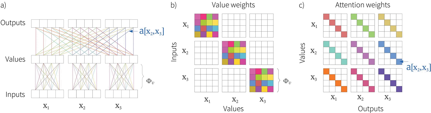
Figure 1. Self attention computation for $I=3$ inputs $\mathbf{x}_{i}$, each of which has dimension $D=4$. a) The input vectors $\mathbf{x}_{i}$ are all operated on independently by the same weights $\boldsymbol\Phi_{v}$ (same color equals same weight) to form the values $\boldsymbol\Phi_{v}\mathbf{x}_{i}$. Each output is a linear combination of these values, where there is a single shared attention weight $a[\mathbf{x}_{i}, \mathbf{x}_{j}]$ that relates the contribution of the $i^{th}$ value to the $j^{th}$ output. b) Matrix showing block sparsity of linear transformation $\boldsymbol\Phi_{v}$ between inputs and values. c) Matrix showing sparsity of attention weights in the linear transformation relating values and outputs.
Computing attention weights
In the previous section, we saw that the outputs are the result of two chained linear transformations; the values $\boldsymbol\Phi_{v}\mathbf{x}_{i}$ are computed independently for each input $\mathbf{x}_{i}$ and these vectors are combined linearly by the attention weights $a[\mathbf{x}_{i},\mathbf{x}_{j}]$. However, the overall self-attention computation is non-linear because the attention weights are themselves non-linear functions of the input.
More specifically, the attention weight $a[\mathbf{x}_{i},\mathbf{x}_{j}]$ depends on the dot-product $(\boldsymbol\Phi_{q}\mathbf{x}_{i})^{T}\boldsymbol\Phi_{k}\mathbf{x}_{j}$ between $\mathbf{x}_{i}$ and $\mathbf{x}_{j}$ after each as been transformed by a different linear transformations $\boldsymbol\Phi_{q}$ and $\boldsymbol\Phi_{k}$ respectively. To complete the computation of the attention weight, these dot-product similarities are passed through a softmax function:
\begin{eqnarray}\label{eq:sattention2} a[\mathbf{x}_{i},\mathbf{x}_{j}] &=& \mbox{softmax}_{j}\left[(\boldsymbol\Phi_{q}\mathbf{x}_{i})^{T}\boldsymbol\Phi_{k}\mathbf{x}_{j} \right]\nonumber\\ &=& \frac{\exp\left[(\boldsymbol\Phi_{q}\mathbf{x}_{i})^{T}\boldsymbol\Phi_{k}\mathbf{x}_{j} \right]}{\sum_{j=1}^{I}\exp\left[(\boldsymbol\Phi_{q}\mathbf{x}_{i})^{T}\boldsymbol\Phi_{k}\mathbf{x}_{j} \right]} \tag{3}\end{eqnarray}
and so for each $\mathbf{x}_{i}$ they are positive and sum to one (figure 2). For obvious reasons, this is known as dot-product self-attention.
The vectors $\boldsymbol\Phi_{q}\mathbf{x}_{i}$ and $\boldsymbol\Phi_{k}\mathbf{x}_{i}$ are known as the queries and keys respectively. These names were inherited from the field of information retrieval and have the following interpretation: the output for input $\mathbf{x}_{i}$ receives a weighted sum of values $\boldsymbol\Phi_v \mathbf{x}_{j}$, where the weights $a[\mathbf{x}_{i}, \mathbf{x}_{j}]$ depend on the similarity between the query vector $\boldsymbol\Phi_q \mathbf{x}_{j}$ and the key vector $\boldsymbol\Phi_k \mathbf{x}_{j}$.
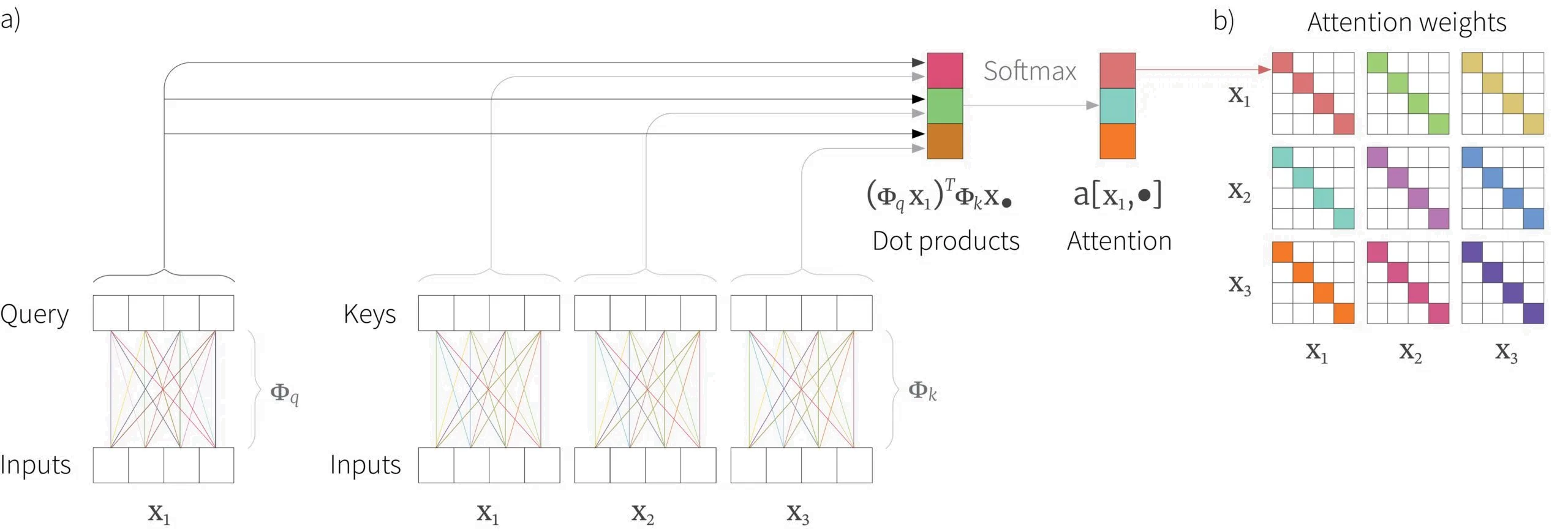
Figure 2. Computing attention weights. A query vector $\boldsymbol\Phi_{q}\mathbf{x}_{i}$ and a key vector $\boldsymbol\Phi_{k}\mathbf{x}_{i}$ are computed for each input $\mathbf{x}_{i}$. Here, we show the computation of the query vector only for input $\mathbf{x}{1}$ but the computation of the key vectors for all three inputs $\mathbf{x}_{1},\mathbf{x}_{2},\mathbf{x}_{3}$. Since, the same parameters $\boldsymbol\Phi_{q}$ and $\boldsymbol\Phi_{k}$ are used for each input, the overall linear transformation for each has the same structure as in figure 1b. The dot product is computed between each query vector and all three keys to give three numbers which are passed through a softmax function which makes them positive and sum to one (b) These three values form three of the weights in the attention weight matrix from figure 1c.
Self-attention summary
To summarize, we see that for input $\mathbf{x}_{i}$, the output is a weighted sum of the same linear transformation $\boldsymbol\Phi_{v}$ of all of the inputs, where these weights are positive and sum to one. The weights depend on a measure of similarity between input $\mathbf{x}_{i}$ and the other inputs. The computation as a whole is non-linear due to the dot-product and softmax operation used to compute these weights. Consequently, there is no need for a pointwise non-linearity like a ReLU.
Note that this mechanism fulfils the requirements that we laid out earlier. First, there is a single shared set of of parameters $\boldsymbol\Phi_{v},\boldsymbol\Phi_{q},\boldsymbol\Phi_{k}$. This is independent of the number of inputs $I$ and so the network can be applied to different sequence lengths. Second, the connections between the inputs (words) depend on the input representations themselves via the computed attention values.
Matrix form
The above computation can be written in a more compact form if we assume that the $I$ inputs $\mathbf{x}_{i}$ are form the rows of the $I\times D$ matrix $\mathbf{x}$:
\begin{equation} \mbox{Sa}[\mathbf{x}] = \mbox{Softmax}[\mathbf{X}\boldsymbol\Phi_{q}(\mathbf{X}\boldsymbol\Phi_{k})^{T}]\mathbf{X}\boldsymbol\Phi_{v}. \tag{4}\end{equation}
where the function $\mbox{Softmax}[\bullet]$ takes a matrix and performs the softmax operation independently on each of its rows (figure 3). Note that here the matrices $\boldsymbol\Phi_{v}, \boldsymbol\Phi_{q}$ and $\boldsymbol\Phi_{k}$ are the transposes of those in the original formulation.
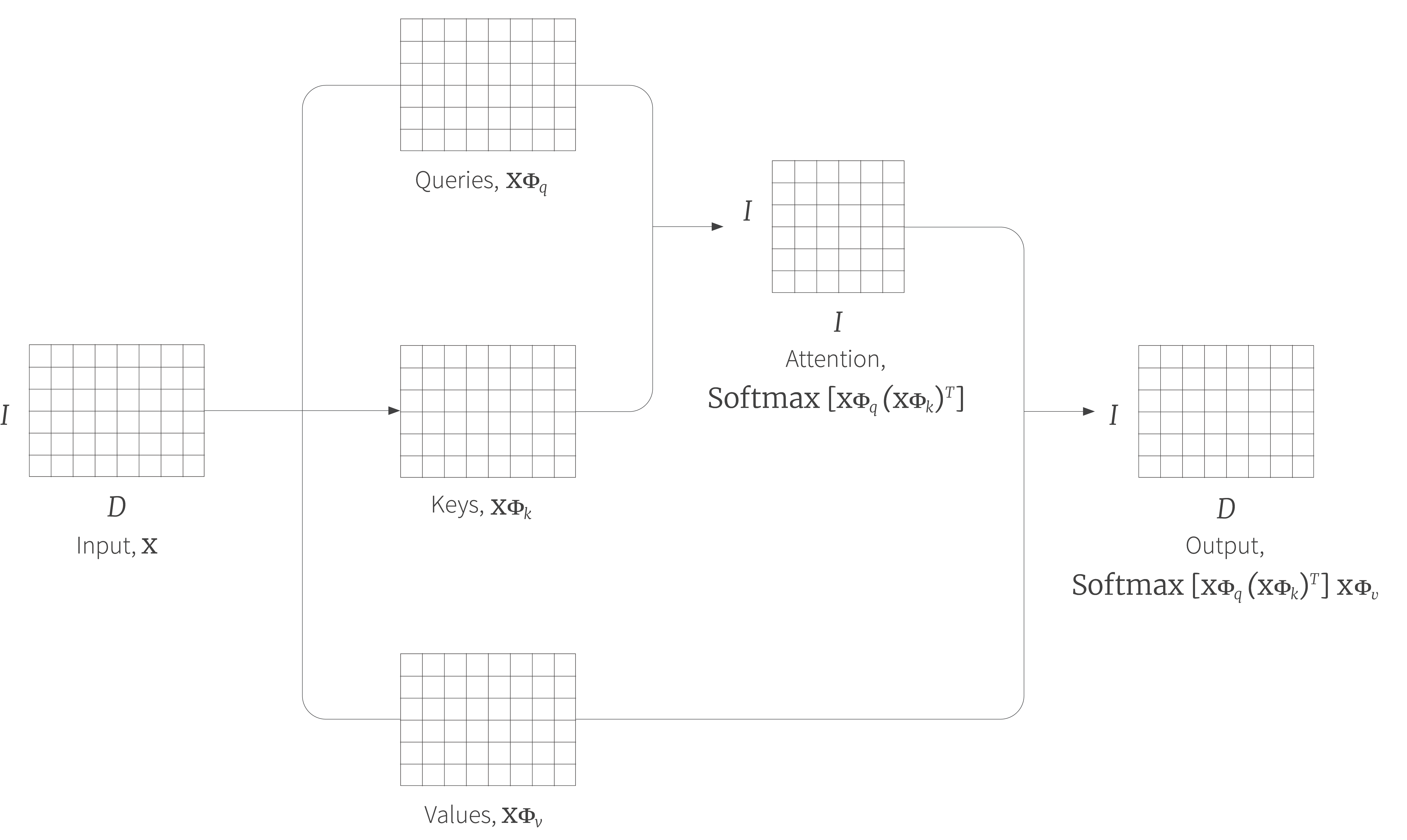
Figure 3. Self attention in matrix form. The self attention mechanism can be implemented efficiently if we store the $I$ input vectors $\mathbf{x}_{i}$ in the rows of a $I\times D$ matrix $\mathbf{X}$. This input $\mathbf{X}$ is operated on separately by the query matrix $\boldsymbol\Phi_{q}$, key matrix $\boldsymbol\Phi_{k}$, and value matrix $\boldsymbol\Phi_{v}$. The dot products can then be computed using matrix multiplication and a softmax operation applied independently to each row of the resulting matrix to compute the attentions. Finally, the values are multiplied by these attentions to create an output of the same size.
Extensions to dot-product self-attention
In the previous section, we described the dot-product self-attention mechanism. Here, we introduce three extensions that are all almost always used in practice.
Positional encoding
Observant readers will have noticed that the above mechanism loses some important information; the computation will be the same, regardless of the order of the inputs $\mathbf{x}_{i}$. However, if the inputs correspond to the words in a sentence, it’s clear that the order matters. To incorporate information about position, we add a matrix $\boldsymbol\Pi$ which is the same size as the input matrix that encodes this information.
The position matrix $\boldsymbol\Pi$ may either be chosen manually or learned. It may be added to the initial word embeddings only or it may be added at every layer of the network. Sometimes it is only added to $\mathbf{x}$ in the computation of the queries and keys. The contents of this vector and other variations will be discussed in detail in part II of this blog; however, the main idea is that there is unique vector added to each input $\mathbf{x}_{i}$ that lets the system know its position in the sequence.
Scaled dot product self-attention
The dot products in the attention computation may have very large magnitudes. This can move the arguments to the softmax function into a region where the largest value dominates to a large degree and consequently, the associated gradients are very small and the model becomes hard to train. To resolve this issue, it is typical to scale the computed attention values by the square root of dimension $d_{q}$ of the queries and keys (i.e., the number of columns in $\boldsymbol\Phi_{q}$ and $\boldsymbol\Phi_{k}$ which must be the same). This gives:
\begin{equation} \mbox{Sa}[\mathbf{x}] =\mbox{Softmax}\left[\frac{(\mathbf{X}\boldsymbol\Phi_{q})(\mathbf{X}\boldsymbol\Phi_{k})^{T}}{\sqrt{d_{q}}}\right]\mathbf{X}\boldsymbol\Phi_{v}. \tag{5}\end{equation}
This is known as scaled dot product self-attention.
Multiple heads
Practitioners usually apply multiple self-attention mechanisms in parallel, and this is known as multi-head self attention. The $h^{th}$ self-attention mechanism or head can be written as:
\begin{equation} \mbox{Sa}_{h}[\mathbf{x}] =\mbox{Softmax}\left[\frac{(\mathbf{X}\boldsymbol\Phi_{qh})(\mathbf{X}\boldsymbol\Phi_{kh})^{T}}{\sqrt{d_{q}}}\right]\mathbf{X}\boldsymbol\Phi_{vh}. \tag{6}\end{equation}
where we have different parameters $\boldsymbol\Phi_{qh}$, $\boldsymbol\Phi_{kh}$ and $\boldsymbol\Phi_{vh}$ for each head. The outputs of these self-attention mechanisms are concatenated and another linear transform $\boldsymbol\Phi_{c}$ is applied to combine them (figure 4):
\begin{equation} \mbox{MhSa}[\mathbf{X}] = \left[\mbox{Sa}_{1}[\mathbf{X}]\;\mbox{Sa}_{2}[\mathbf{X}]\;\ldots\;\mbox{Sa}_{H}[\mathbf{X}] \right]\boldsymbol\Phi_{c}. \tag{7}\end{equation}
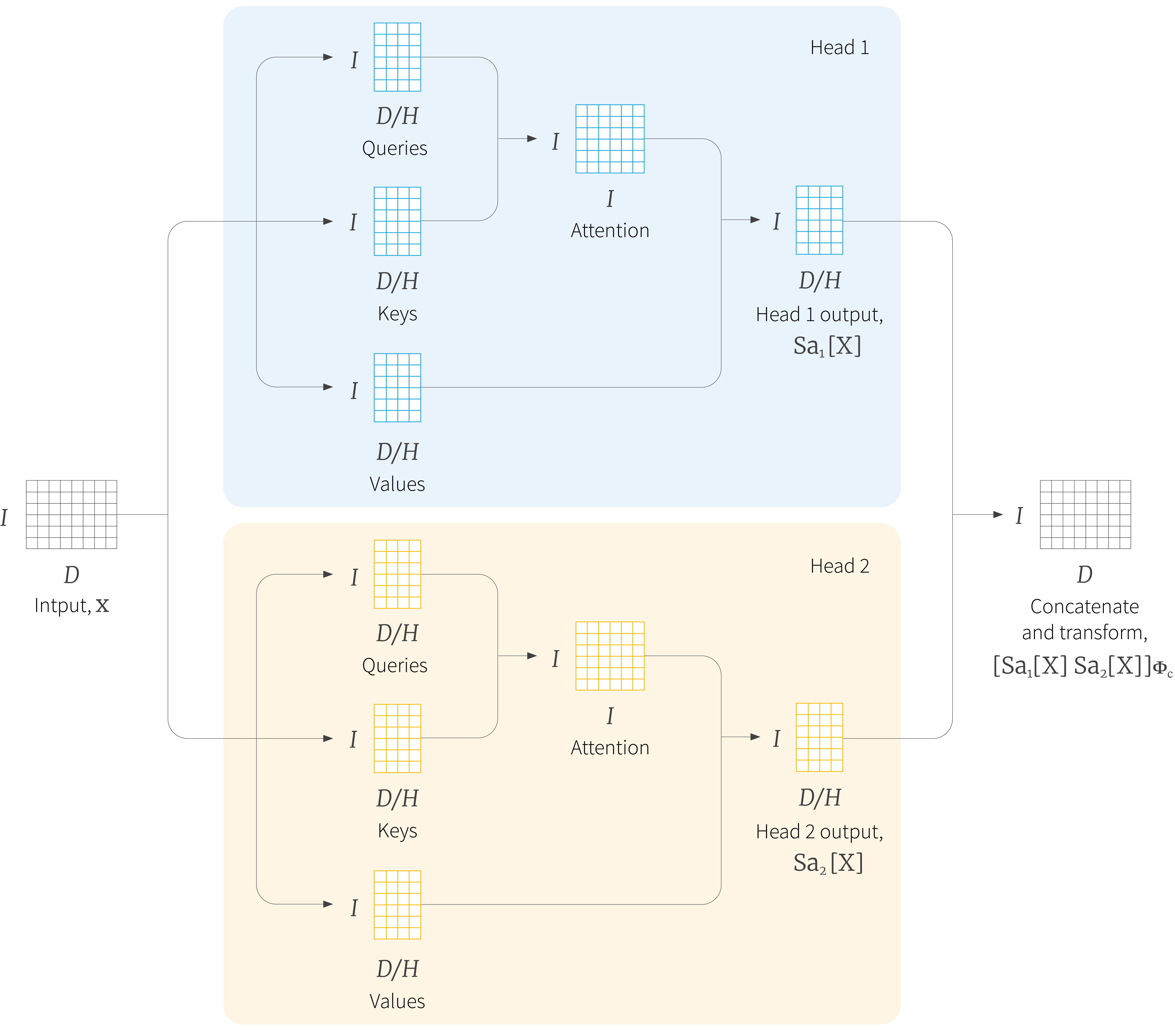
Figure 4. Muti-head self-attention. Self-attention generally occurs in parallel across multiple “heads”. Each head has its own queries, keys, and values. In this figure two heads are depicted, in the red and blue boxes respectively. The outputs of each head are concatenated together and a further linear transformation $\boldsymbol\Phi_{c}$ is applied to recombine them. Typically, if the dimension of the inputs $\mathbf{x}_{i}$ is $D$ and there are $H$ heads, then the values, queries, and keys will all be of size $D/H$ as this allows for an efficient implementation in which all of the queries, keys and values can be computed by a single matrix multiplication (not shown).
This appears to be necessary to make the transformer work well in practice. It has been speculated that multiple heads make the self-attention network more robust to bad initializations. The fact that trained models only seem to depend on a subset of the heads lends credence to this speculation.
Transformer layers
Self-attention is just one part of a larger transformer layer. This layer consists of a multi-head self-attention unit (which allows the word representations to interact with each other) followed by a fully connected network $\mbox{mlp}[\mathbf{x}_{i}]$ (that operates separately on each word representation). Both of these units are residual networks (i.e., their output is added back to the original input). In addition, it is typical to add a LayerNorm operation after both the self-attention and fully connected networks. The complete layer can be described by the following series of operations:
\begin{eqnarray} \mathbf{x} &\leftarrow& \mathbf{x} + \mbox{MhSa}[\mathbf{x}] \nonumber \\ \mathbf{x} &\leftarrow& \mbox{Layernorm}[\mathbf{x}] \hspace{3cm}\nonumber\\ \mathbf{x}_{i} &\leftarrow& \mathbf{x}_{i}+\mbox{mlp}[\mathbf{x}_{i}] \hspace{3.6cm}\forall\; i\in\{1\ldots I\}\nonumber\\ \mathbf{x} &\leftarrow& \mbox{Layernorm}[\mathbf{x}], \tag{8}\end{eqnarray}
where the column vectors $\mathbf{x}_{i}$ are transposed and form the rows of the full data matrix $\mathbf{x}$ in the first stage. In a real system, the data would pass through a series of these layers.
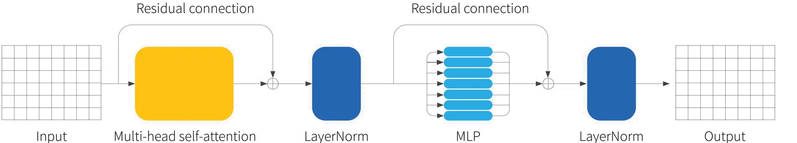
Figure 5. The transformer layer. The input consists of a $I\times D$ matrix containing the $D$ dimensional word embeddings for each of the $I$ input tokens. The output is a matrix of the same size. The transformer layer consists of a series of operations. First, there is a multi-head attention block which allows the word embeddings to interact with one another. This is in a residual network, so the original inputs are added back to the output. Second, a layer norm operation is applied. Third, there is a second residual network where the same two-layer fully-connected neural network is applied to each word representation separately. Finally, layer-norm is applied again.
How transformers are used in NLP
Now that we have a good understanding of self-attention and the transformer layer, let’s walk through a typical modern NLP processing pipeline.
Tokenization
A text processing pipeline begins with a tokenizer. This splits the text into a vocabulary of smaller constituent units (tokens) that can be processed by the subsequent network. In the discussion above, we have implied that these are words, but there are a several difficulties with this.
- It’s inevitable that some words (e.g., names) will not be in the vocabulary.
- It’s not clear how to handle punctuation, but this is important. If a sentence ends in a question mark, then we need to encode this information.
- The vocabulary would need different tokens for versions of the same word with different suffixes (e.g., walk, walks, walked, walking) and there is no way to make clear that these variations are related.
One approach would be just to use letters and punctuation marks as the vocabulary, but this would mean splitting text into a large number of very small parts and requiring the subsequent network to re-learn the relations between them.
In practice, a compromise between using letters and full words is used, and the final vocabulary will include both common words and short parts of words from which larger and less frequent words can be composed. The vocabulary is computed using a method such as byte pair encoding that uses ideas from text compression methods; essentially it greedily merges commonly-occurring sub-strings based on their frequency. This type of approach is known as a sub-word tokenizer.
Embeddings
Each different token within the vocabulary is mapped to a word embedding. Importantly, the same token always maps to the same embedding. These embeddings are learned along with the rest of unknown parameters in the network. A typical embedding size is 1024 and a typical total vocabulary size is 30,000, and so even before the main network, there are a lot of parameters to learn.
These embeddings are then collected to form the rows of the input matrix $\mathbf{x}$ and the positional encoding $\boldsymbol\Pi$ may be added at this stage.
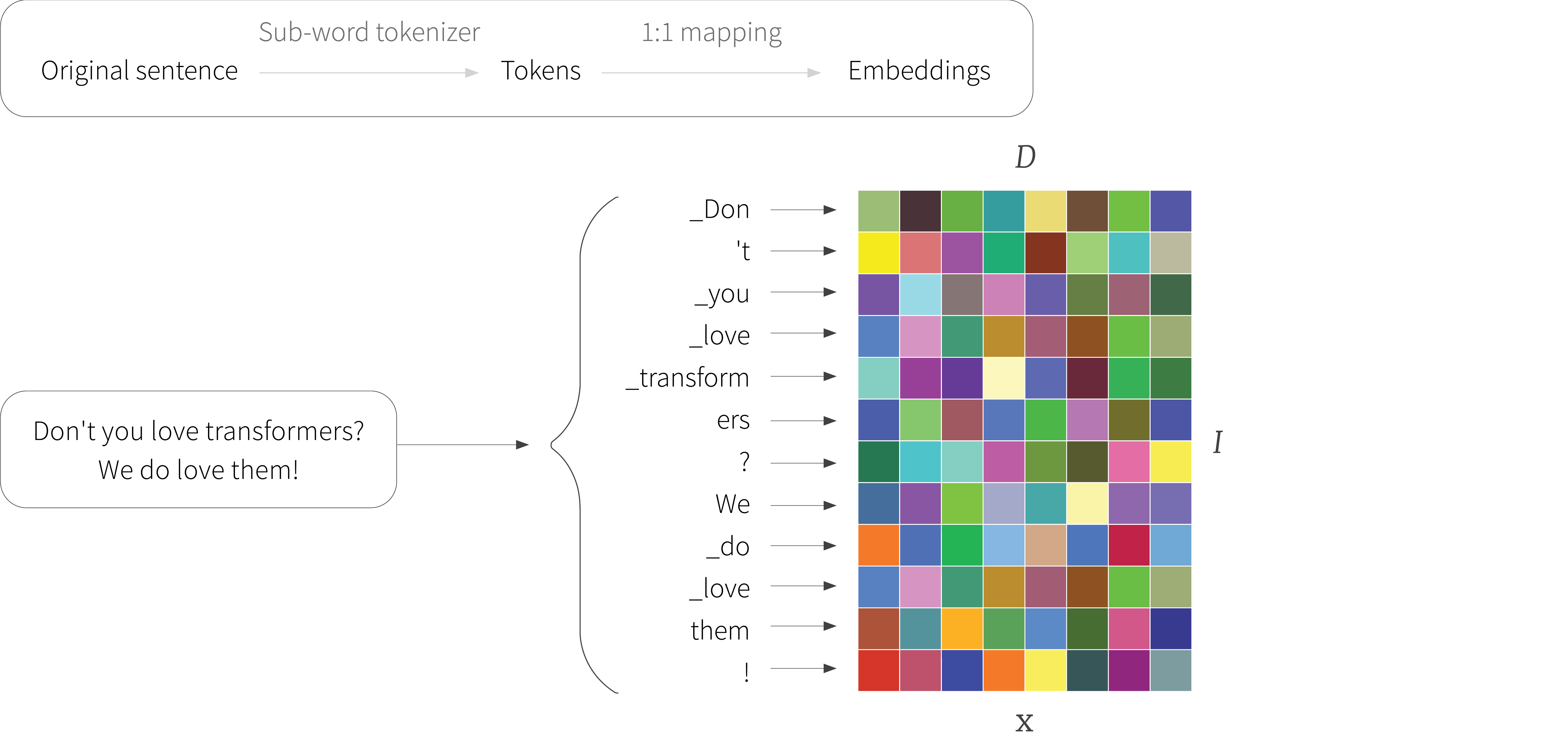
Figure 6. Sub-word tokenization. The original sentence is broken down into a series of tokens, each of which denotes a word, sub-word, or punctuation mark. Note that white space is represented using underscores. Common words like $\textcolor[rgb]{0.502, 0.369, 0.0}{\text{_we}}$ have tokens associated with them but the unusual word $\textcolor[rgb]{0.502, 0.369, 0.0}{\text{_transformers}}$ must be split into sub-words $\textcolor[rgb]{0.502, 0.369, 0.0}{\text{_transform}}$ and $\textcolor[rgb]{0.502, 0.369, 0.0}{\text{ers}}$. Each of the $I$ tokens is mapped to an embedding of length $D$ and these form the rows of the input matrix $\mathbf{X}$. These embeddings are unique to each token; colors depict different values, and notice that the two rows representing the token $\textcolor[rgb]{0.502, 0.369, 0.0}{\text{_love}}$ are identical. These embeddings are usually learned along with the other parameters of the transformer.
Transformer layers
Finally, the input embedding matrix $\mathbf{X}$ is passed to a series of transformer layers, which we’ll refer to as a transformer network from now on. There are three main types of transformer network. First, a transformer network can be used as an encoder. Here, the goal is to transform the text into a representation that can support a variety of language tasks, such as sentiment analysis or question answering. An example of an encoder model is the BERT model.
Second, a transformer network can be used as a decoder. Here, the goal of the network is to generate a new token that continues the input text. An example of a decoder model is GPT3.
Finally, transformer networks can be used to build encoder-decoder models. These are used in sequence to sequence models, which take one text string and convert them to another text string. For example, in machine translation, an input sentence in English might be processed by the encoder. The decoder then generates the translated sentence in French. An example of an encoder-decoder model is the paper where transformers were first introduced.
We’ll now consider each of these three variations in turn.
Encoder model example: BERT
BERT is an encoder model that uses s a vocabulary of 30,000 tokens. The tokens are converted to 1024 dimensional word embeddings and passed through 24 transformer layers. In each of these is a self-attention layer with 16 heads, and for each head the queries, keys, and values are of dimension 64 (i.e., the matrices $\boldsymbol\Phi_{vh},\boldsymbol\Phi_{qh},\boldsymbol\Phi_{kh}$ are of size $1024\times 64$). The dimension of the hidden layer in the neural network layer of the transformer is 4096. The total number of parameters is $\sim 340$ million. This sounds like a lot, but is tiny by modern standards.
Encoder models are trained in two stages. During pre-training, the parameters of the transformer architecture are learned using self-supervision from a large corpus of text. The goal here is for the model to learn general information about the statistics of language. In the fine-tuning stage, the resulting network is adapted to solve a particular task, using a smaller body of supervised training data. We’ll now discuss each of these stages in turn for the BERT model.
Pre-training
In the pre-training stage, the network is trained using self-supervision. This allows the use of enormous amounts of data, without the need for manual labels. For BERT, the self-supervision task consists of predicting missing words from sentences from a large internet corpus (figure 7)1. During training, the maximum input length was 512 tokens and the batch size is 256. The system is trained for 1,000,000 steps which is roughly 50 epochs of the 3.3 billion word corpus.
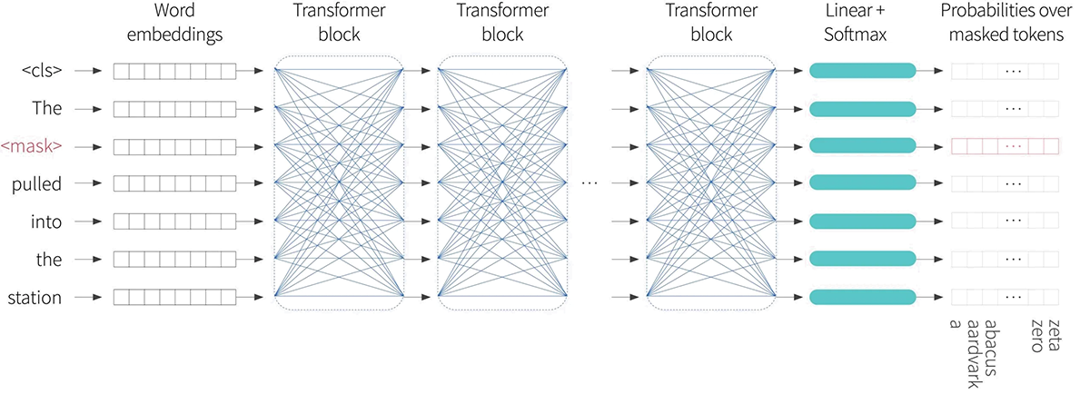
Figure 7. Pre-training for BERT-like encoder. The input tokens (and a special $<$cls$>$ token denoting the start of the sequence) are converted to word embeddings and passed through a series of transformer layers (blue connections indicate that every token attends to every other token in these layers). A small fraction of the input tokens are replaced at random with a generic $<$mask$>$ token. In pre-training, the goal is to predict the missing word. As such, the output embeddings are used to predict a probability over the vocabulary and the log likelihood of the ground truth masked tokens is used as the objective function. This task has the advantage that is uses both the left and right context to predict the missing word, but has the disadvantage that it does not make very efficient use of data; in this case seven tokens need to be processed to add a single term to the objective function.
Trying to predict missing words forces the transformer network to understand something of the syntax of the language. For example, that it might learn that the adjective red is often found before nouns like house or car but never before a verb like shout. It also allows the model to learn some superficial common sense about the world. For example, after training, the model will assign a higher probability to the missing word train in the sentence The <mask> pulled into the station, than it would to the word peanut. However, there are persuasive arguments that the degree of “understanding” that this type of model can ever have is limited.
Fine-tuning
In the fine-tuning stage, the parameters of the model are adjusted to specialize it to a particular task. This usually involves adding an extra layer on top of the transformer network, to convert the collection of vectors $\mathbf{x}_{1},\ldots \mathbf{x}_{I}$ associated with the input tokens to the desired format of the output. Examples include:
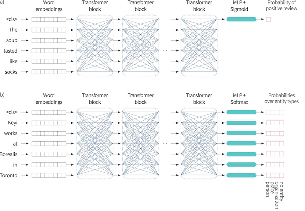
Figure 8. After pre-training using the masked-word task, the encoder is fine-tuned using manually labelled data to solve a particular task. Usually, a linear transformation or a multi-layer perceptron (MLP) is added to the end of the encoder to produce whatever output is required for the task. a) Example of a text classification task. In this sentiment classification task, the $<$cls$>$ token embedding is used to predict the probability that the review is positive. b) Example of a word- lassification task. In this entity recognition task, the embedding for each individual word is used to predict whether the word is person, place, organization, or is not an entity.
Text classification: In BERT, there is a special token known as the $<$cls$>$ token (short for classification token) that is placed at the start of each string during pre-training. For text classification tasks like sentiment analysis, the vector associated with this string is mapped to a single number and passed through a logistic sigmoid. This creates a number between 0 and 1 that can be interpreted as the probability that the sentiment is positive and the system is fine-tuned to maximize this correct probability (figure 8a).
Word classification: In named entity recognition, the goal is to classify each individual word as an entity type (e.g., person, place, organization, or no-entity). To this end, the vector $\mathbf{x}_{i}$ associated with each token in the input sequence is mapped to a $K\times 1$ vector where $K$ is the entity type (figure 8a) and the system is fine tuned to maximize these probabilities (figure 8b).
Text span prediction: In the SQuAD 1.1 question answering task, both the question and a passage from Wikipedia containing the answer are input into the system. BERT is then used to predict the text span in the passage that contains the answer. Each token associated with the Wikipedia passage maps to two numbers, that indicate how likely it is that the text span begins and ends at this location. The resulting two sets of numbers are put through two softmax functions and the probability of any text span being the answer can then be derived by combining the probability of starting and ending at the appropriate places.
Decoder model example: GPT3
In this section, we present a high-level description of GPT3 which is an example of a transformer decoder model. The basic architecture is extremely similar to the encoder model in that it consists of a series of transformer layers that operate on learned word embeddings. However, the goal is different. The encoder aimed to build a representation of the text that could be fine-tuned to solve a more specific NLP task. However, the decoder has one purpose which is to generate the next token in a provided sequence. By iterating this procedure, the model can produce a body of coherent text.
Language modeling
More specifically, GPT3 constructs a language model. For any sentence it aims to model the joint probability $Pr(t_1,t_2,\ldots t_{N})$ of the $N$ observed tokens and it does this by factorizing this joint probability into an auto-regressive sequence:
\begin{equation} Pr(t_{1},t_{2},\ldots t_{N}) = \prod_{n=1}^{N}Pr(t_{n}|t_{1}\ldots t_{n-1}). \tag{9}\end{equation}
This is easiest to understand with a concrete example. Consider the sentence It takes great personal courage to let yourself appear weak. For simplicity, let’s assume that the tokens are the full words. The probability of the full sentence is:
$Pr$(It takes great personal courage to let yourself appear weak) $=$ $Pr$(It) $\cdot$ $Pr$(takes$|$It) $\cdot$ $Pr$(great$|$It takes) $\cdot$ $Pr$(courage$|$It takes great) $\cdot$
$Pr$(to$|$It takes great courage) $\cdot$ $Pr$(let$|$It takes great courage to) $\cdot$
$Pr$(yourself$|$It takes great courage to let) $\cdot$
$Pr$(appear$|$It takes great courage to let yourself) $\cdot$
$Pr$(weak$|$It takes great courage to let yourself appear). (10)
This demonstrates the connection between the probabilistic formulation of the cost function and the next token prediction task.
Masked self-attention
When we train a decoder model, we aim to maximize the log-probability of the input text under the auto-regressive language model. Ideally, we would like to pass in the whole sentence and compute all of the log probabilities and their gradients simultaneously. However, this poses a problem; if we pass in the full sentence, then the term computing $\log$ $[$ $Pr$(great$|$It takes) $]$ will have access to both the answer great and also the right context courage to let yourself appear weak.
To see how to avoid this problem, recall that in a transformer network, the tokens only interact in the self-attention layers. This implies that the problem can be resolved by ensuring that the attention to the answer and the right context are zero. This can be achieved by setting the appropriate dot products to negative infinity before they are passed through the $\mbox{softmax}[\bullet]$ function. This idea is known as masked self-attention.
The overall decoder transformer network operates as follows. The input text is tokenized and the tokens are converted to embeddings. The embeddings are passed into the transformer network, but now the transformer layers use masked self-attention so that they can only attend to the current and previous tokens. You can think of each of the output embeddings as representing a partial sentence, and for each the goal is is to predict the next token in the sequence. Consequently, after the transformer layers, a linear layer maps each word embedding to the size of the vocabulary, followed by a $\mbox{softmax}[\bullet]$ function that converts these values to probabilities. We aim to maximize sum of the log probabilities of the next token in the ground truth sequence at every position (figure 9).
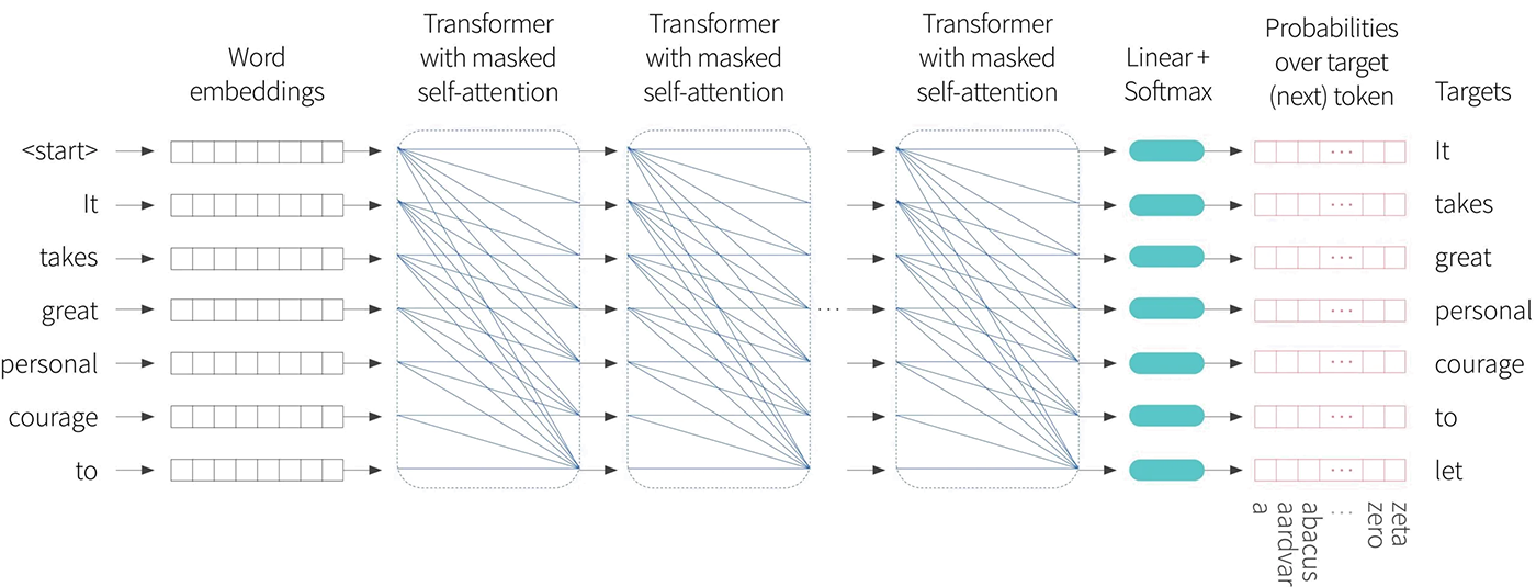
Figure 9. GPT3-type decoder network. The tokens are mapped to word embeddings with a special $<$start$>$ token at the beginning of the sequence. The embeddings are passed through a series of transformers that use masked self-attention in which each position in the sentence can only attend to its own embedding and the embeddings of tokens earlier in the sequence (blue connections). The goal at each position is to maximize the probability of the ground truth token that follows in the sequence. In other words at position one, we want to maximize the probability of the token $\textcolor[rgb]{0.502, 0.369, 0.0}{\text{It}}$, at position two we want to maximize the probability of the token $\textcolor[rgb]{0.502, 0.369, 0.0}{\text{takes}}$ and so on. The masked self-attention ensure that the system cannot cheat by looking at subsequent inputs. This system has the advantage that it makes more efficient use of the data than BERT since every word contributes a term to the cost function. However, it has the disadvantage that it only uses the left-context of each word to predict it.
Generating text from a decoder
To generate from the model, we start with an input sequence of text (which might be just the special $<$start$>$ token) and feed this into the network which then outputs the probability of the next token. We can then either pick the most likely token or sample from this probability distribution. The new extended sequence can be fed back into the decoder network which outputs the probability distribution over the next token and in this way, we can generate large bodies of text. The computation can be made quite efficient as prior embeddings do not interact with subsequent ones due to the masked self-attention and so a lot of the earlier computation can be recycled as we generate subsequent tokens.
In practice, there are many strategies such as beam-search and top-K sampling that can be added to help make the output text more coherent. These are discussed in detail in our previous blog on natural language generation. Here’s an example of completing text from the GPT2 model:
RBC Borealis is a great place to work because there are a lot of people there that are passionate about this kind of technology, like me. There are some challenges for developers but it also gives us a great opportunity to work on different problems.
where the text provided to the model is in brown and the generated text in in blue.
GPT3 and few-shot learning
GPT3 applies these ideas on a massive scale. The sequence lengths are 2048 tokens long and since multiple spans of 2048 tokens are processed at once, the total batch size is 3.2 million tokens. There are 96 transformer layers (some of which implement a sparse version of attention), each of which processes a word embedding of size 12288. There are 96 heads in the self-attention layers and the value, query and key dimension is 128. It is trained with 300 billion tokens and learns a total of 175 billion parameters. It is interesting to note that since text is extremely compressible, it actually contains more than enough capacity to memorize the entire data set.
One surprising property of learning a model on this scale is that it can perform many tasks without the need for fine-tuning. If we provide several examples of correct question answer pairs, and then another question, it can often answer the final question correctly just by completing the sequence. One example of this is correcting English grammar:
Poor English input: I eated the purple berries.
Good English output: I ate the purple berries.
Poor English input: Thank you for picking me as your designer. I’d appreciate it.
Good English output: Thank you for choosing me as your designer. I appreciate it.
Poor English input: The mentioned changes have done. or I did the alteration that you requested. or I changed things you wanted and did the modifications.
Good English output: The requested changes have been made. or I made the alteration that you requested. or I changed things you wanted and made the modifications.
Poor English input: I’d be more than happy to work with you in another project.
Good English output: I’d be more than happy to work with you on another project.
The text containing the paired examples in brown was provided as context for GPT3 and the system then generated the correct answer in blue. This phenomenon extends to many situations including generating code snippets based on natural language descriptions, simple arithmetic, translating between languages, answering questions about text passages and many more. Consequently, it is argued that enormous language models are few-shot learners; they can learn to do novel tasks based on just a few examples. However, in practice the performance is erratic and it is not clear the extent to which it is extrapolating from learned examples rather than merely interpolating, or even copying verbatim.
Encoder-decoder models
The original transformer paper focused on translation between languages, which is an example of a sequence-to-sequence task. Their original architecture was an encoder-decoder model that (as the name suggests) combines both encoder and decoder models.
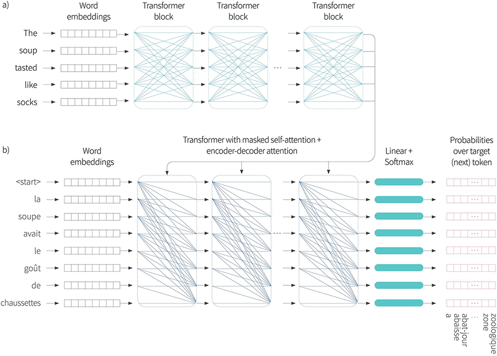
Figure 10. Encoder-decoder architecture. Two sequences are input to the system and with the goal of learning to translate the first sentence into the second. a) The first sentence is passed through a standard encoder. b) The second sentence is passed through a decoder that uses masked self attention, but also attends to the output embeddings of the encoder using encoder-decoder attention. The cost function is the same as for the decoder; we want to maximize the probability of the next word in the output sequence.
Consider the example of translating from English to French. The encoder receives the sentence in English and processes it through a series of transformer layers to create an output representation for each token. The decoder receives the sentence in French and processes through a series of transformer layers that use masked self-attention. However, these transformer layers also attend to the output of the encoder. Consequently, each French output word conditioned not only on the previous output words, but also on the entire English sentence that it is translating (figure 10).
In practice this is achieved by modifying the transformer layer. The original transformer layer in the decoder (figure 5) consisted of a masked self-attention layer followed by a multi-layer perceptron applied individually to each embedding. In between these we now introduce a second attention layer, in which the embeddings attend to the output embeddings from the encoder. This uses a version of self-attention where the queries $\mathbf{X}_{d}\boldsymbol\Phi_{q}$ are computed from the decoder embeddings $\mathbf{X}_{d}$, and the keys $\mathbf{X}_{e}\boldsymbol\Phi_{k}$ and values $\mathbf{X}_{e}\boldsymbol\Phi_{v}$ are generated from the encoder embeddings $\mathbf{X}_{e}$:
\begin{equation}\mbox{ Sa}[\mathbf{X}_{d},\mathbf{x}_{e}] = \mbox{Softmax}[\mathbf{X}_{d}\boldsymbol\Phi_{q}(\mathbf{X}_{e}\boldsymbol\Phi_{k})^{T}]\mathbf{X}_{e}\boldsymbol\Phi_{v}. \tag{11}\end{equation}
This is known as encoder-decoder attention (figure 11).
Figure 11. Encoder-decoder self-attention. The flow of computation is the same as for vanilla self-attention, but now the queries are calculated from the decoder embeddings $\mathbf{X}_{d}$, but the keys and values are calculated from the encoder embeddings $\mathbf{X}_{e}$.
Summary
In this blog, we introduced the idea of self-attention and then described how this fits into the transformer architecture. We then presented the encoder, decoder, and encoder-decoder versions of this architecture. We’ve seen that the transformer operates on sets of high-dimensional embeddings. It has a low computational complexity per layer and much of the computation can performed in parallel, using the matrix form. Since every input embedding interacts with every other, it can describe long-range dependencies in text. It is these characteristics that have allowed transformers to be applied in massive systems like GPT3.
In the second part of the blog we will discuss extensions of the basic transformer model. In particular, we will expand on methods to encode the position of tokens and methods to extend transformers to process very long sequences. We’ll also discuss how the transformer architecture relates to other models. Finally, in the third part of this series, we will discuss the details of how to train transformer models successfully.
1 BERT also used a secondary task which involved predicting whether two sentences were originally adjacent in the text or not, but this only marginally improved performance.
News
Meet Turing by RBC Borealis, an AI-powered text to SQL database interface
Work with Us!
Impressed by the work of the team? RBC Borealis is looking to hire for various roles across different teams. Visit our career page now and discover opportunities to join similar impactful projects!
Careers at RBC Borealis