
Introduction
Reinforcement learning (RL) can now produce super-human performance on a variety of tasks, including board games such as chess and go, video games, and multi-player games such as poker. However, current algorithms require enormous quantities of data to learn these tasks. For example, OpenAI Five generates 180 years of gameplay data per day, and AlphaStar used 200 years of Starcraft II gameplay data.
It follows that one of the biggest challenges for RL is sample efficiency. In many realistic scenarios, the reward signals are sparse, delayed or noisy which makes learning particularly inefficient; most of the collected experiences do not produce a learning signal. This problem is exacerbated because RL simultaneously learns both the policy (i.e., to make decisions) and the representation on which these decisions are based. Until the representation is reasonable, the system will be unable to develop a sensible policy.
This article focuses on the use of auxiliary tasks to improve the speed of learning. These are additional tasks that are learned simultaneously with the main RL goal and that generate a more consistent learning signal. The system uses these signals to learn a shared representation and hence speed up the progress on the main RL task.
What are Auxiliary Tasks?
An auxiliary task is an additional cost-function that an RL agent can predict and observe from the environment in a self-supervised fashion. This means that losses are defined via surrogate annotations that are synthesized from unlabeled inputs, even in the absence of a strong reward signal.
Auxiliary tasks usually consist of estimating quantities that are relevant to solving the main RL problem. For example, we might estimate depth in a navigation task. However, in other cases, they are be more general. For example, we might try to predict how close the agent is to a terminal state. Accordingly, they may take the form of classification and regression algorithms or alternatively may maximize reinforcement learning objectives.
We note that auxiliary tasks are different from model-based RL. Here, a model of how the environment transitions between states given the actions is used to support planning (Oh et al. 2015; Leibfried et al. 2016) and hence ultimately to directly improve the main RL objective. In contrast, auxiliary tasks do not directly improve the main RL objective, but are used to facilitate the representation learning process (Bellemare et al. 2019) and improve learning stability (Jaderberg et al. 2017).
History of auxiliary tasks
Auxiliary tasks were originally developed for neural networks and referred to as hints. Suddarth & Kergosien (1990) argued that for the hint to be effective, it needs to “special relationship with the original input-output being learned.” They demonstrated that adding auxiliary tasks to a minimal neural network effectively removed local minima.
The idea of adding supplementary cost functions was first used in reinforcement learning by Sutton et al. (2011) in the form of general value functions (GVFs). As the name suggests, GVFs are similar to the well-known value functions of reinforcement learning. However, instead of caring about environmental rewards, they consider other signals. They differ from auxiliary tasks in that they usually predict long term features. Hence, they employ summation across multiple time-steps similar to the state-value computation from rewards in standard RL.
Implementing auxiliary tasks
Auxiliary tasks are naturally and succinctly implemented by splitting the last layer of the network into multiple parts (heads), each working on a different task. The multiple heads propagate errors back to the shared part of the network, which forms the representations that support all the tasks (Sutton & Barto 2018).
To see how this works in practice, we’ll consider Asynchronous Advantage Actor-Critic (A3C) (Mnih et al. 2016), which is a popular and representative actor-critic algorithm. The loss function of A3C is composed of two terms: the policy loss (actor), $\mathcal{L}_{\boldsymbol\pi}$, and the value loss (critic), $\mathcal{L}_{v}$. An entropy loss $H[\boldsymbol\pi]$ for the policy $\boldsymbol\pi$, is also commonly added. This helps discouraging premature convergence to sub-optimal deterministic policies (Mnih et al. 2016). The complete loss function is given by:
\begin{equation}\mathcal{L}_{\text{A3C}} = \lambda_v \mathcal{L}_{v} + \lambda_{\pi} \mathcal{L}_{\pi} – \lambda_{H} \mathbb{E}_{s \sim \pi} \left[H[\boldsymbol\pi[s]]\right]\tag{1}\end{equation}
where $s$ is the state and scalars $\lambda_{v},\lambda_{\boldsymbol\pi}$, and $\lambda_{H}$ weight the component losses.

Figure 1. Auxiliary tasks for an actor critic model. The network has a shared set of convolutional and fully connected layers. These provide input for three heads, corresponding to value prediction, policy prediction and auxiliary task prediction. Each head contributes to the final loss function.
Auxiliary tasks are introduced to A3C via the Unsupervised Reinforcement and Auxiliary Learning (UNREAL) framework (Jaderberg et al. 2017). UNREAL optimizes the loss function:
\begin{equation}\mathcal{L}_{\text{UNREAL}} = \mathcal{L}_{\text{A3C}} + \sum_i \lambda_{AT_i} \mathcal{L}_{AT_i}\tag{2}\end{equation}
that combines the A3C loss, $\mathcal{L}_{\text{A3C}}$, together with auxiliary task losses $\mathcal{L}_{AT_i}$, where $\lambda_{AT_i}$ are weight terms (Figure 1). For a single auxiliary task, the loss computation code might look like:
def loss_func_a3c(s, a, v_t):
        # Compute logits from policy head and values from the value head
        self.train()
        logits, values = self.forward(s)
        # Critic loss computation
        td = 0.5*(v_t - values)
        c_loss = td.pow(2)
        # Actor loss
        probs = F.softmax(logits, dim=1)
        m = self.distribution(probs)
        exp_v = m.log_prob(a) * td.detach()
        a_loss = -exp_v
        # Entropy loss
        ent_loss = -(F.log_softmax(logits, dim=1) * F.softmax(logits, dim=1)).sum(1)
        # Computing total loss
        total_loss = (CRITIC_LOSS_W * c_loss + ACTOR_LOSS_W * a_loss - ENT_LOSS_W * ent_loss).mean()
        # Auxiliary task loss
        aux_task_loss = aux_task_computation()
        #Computing total loss
        total_loss = (AUX_TASK_WEIGHT_LOSS * aux_task_loss + a3c_loss).mean()
The use of auxiliary tasks is not limited to actor-critic algorithms; they have also been implemented on top of Q-learning algorithms such as DRQN (Hausknecht & Stone 2015). For example, Lample & Chaplot (2017) extended the DRQN architecture with another head used to predict game features. In this case, the loss is the standard DRQN loss and the cross-entropy loss of the auxiliary task.
Examples of Auxiliary Tasks
We now consider five different auxiliary tasks that have obtained good results in various RL domains. We provide insights as to the applicability of these tasks.
Task #1: Terminal prediction
Sutton et al. (2011) speculated:
“Suppose we are playing a game for which base terminal rewards are +1 for winning and -1 for losing. In addition to this, we might pose an independent question about how many more moves the game will last. This could be posed as a general value function.“
The first part of the quote refers to the standard RL problem where we learn to maximize rewards (winning the game). The second part describes an auxiliary task in which we predict how many moves remain before termination.
Kartal et al. (2019) investigated this idea of terminal prediction. The agent predicts how close it is to a terminal state while learning the standard policy, with the goal of facilitating representation learning. Kartal et al. (2019) added this auxiliary task to A3C and named this A3C-TP. The architecture was identical to A3C, except for the addition of the terminal state prediction head.
The loss $\mathcal{L}_{TP}$ for the terminal state prediction is the mean squared error between the estimated closeness $\hat{y}$ to a terminal state of any given state and target values $y$ approximately computed from completed episodes:
\begin{equation}\mathcal{L}_{TP}= \frac{1}{N} \sum_{i=0}^{N}(y_{i} – \hat{y}_{i})^2\tag{3}\end{equation}
where $N$ represents the episode length during training. The target for the $i^{th}$ state is approximated with $y_{i} = i/N $ implying $y_{N}=1$ for the actual terminal state and $y_{0}=0$ for the initial state for each episode.
Kartal et al. (2019) initially used the actual current episode length for $N$ to compute the targets $y_{i}$. However, this delays access to the labels until the episode is over and did not provide significant benefit in practice. As an alternative, they approximate the current episode length by the running average of episode lengths computed from the most recent $100$ episodes, which provides a dense signal.1 This improves learning performance, and is memory efficient for distributed on-policy deep RL as CPU workers do not have to retain the computation graph until episode termination to compute terminal prediction loss.
Since terminal prediction targets are computed in a self-supervised fashion, they have the advantage that they are independent of reward sparsity or any other domain dynamics that might render representation learning challenging (such as drastic changes in domain visuals, which happen in some Atari games). However, terminal prediction is applicable only for episodic environments.
Task #2: Agent modeling
Agent modeling (Hernandez-Leal et al. 2019) is an auxiliary task that is designed to work in a multi-agent setting. It takes ideas from game theory and in particular from the concept of best response: the strategy that produces the most favorable outcome for a player, taking other players’ strategies as given.
The goal of agent modeling is to learn other agents’ policies while itself learning a policy. For example, consider a game in which you face an opponent. Here, learning the opponent’s behavior is useful to develop a strategy against it. However, agent modeling is not limited to only opponents; it can also model teammates, and can be applied to an arbitrary number of them.
There are two main approaches to implementing the agent modeling task. The first uses the conventional approach of adding new heads for the auxiliary task to a shared network base, as discussed in previous sections. The second uses a more sophisticated architecture in which latent features from the auxiliary network are used as inputs to the main value/policy prediction stream. We consider each in turn.
Agent modeling with parameter sharing (AMS)
In this scheme, agents share the same network base, but the outputs represent different agent actions (Foerster et al. 2017). The goal is to predict opponent policies as well as the standard actor and critic, with the key characteristic that the previous layers share parameters (Figure 2a).
This architecture builds on the concept of parameter sharing where the idea is to perform centralized learning:
The AMS architecture uses the loss function:
\begin{equation}\mathcal{L}_{\text{AMS}}= \mathcal{L}_{\text{A3C}} + \frac{1}{\mathcal{N}} \sum_i^{\mathcal{N}} \lambda_{AM_i} \mathcal{L}_{AM_i}\tag{4}\end{equation}
where $\lambda_{AM_i}$ is a weight term and $\mathcal{L}_{AM_i}$ is the auxiliary loss for opponent $i$:
\begin{equation}\mathcal{L}_{AM_i}= -\frac{1}{M} \sum_j^M \sum_{k}^{K} a^j_{ik} \log [\hat{a}^j_{ik}\tag{5}\end{equation}
which is the cross entropy loss between the observed one-hot encoded opponent action, $\mathbf{a}^j_{i}$, and the prediction over opponent actions, $\hat{\mathbf{a}}^j_{i}$. Here $i$ indexes the opponents, $j$ indexes time for a trajectory of length $M$, and $k$ indexes the $K$ possible actions.
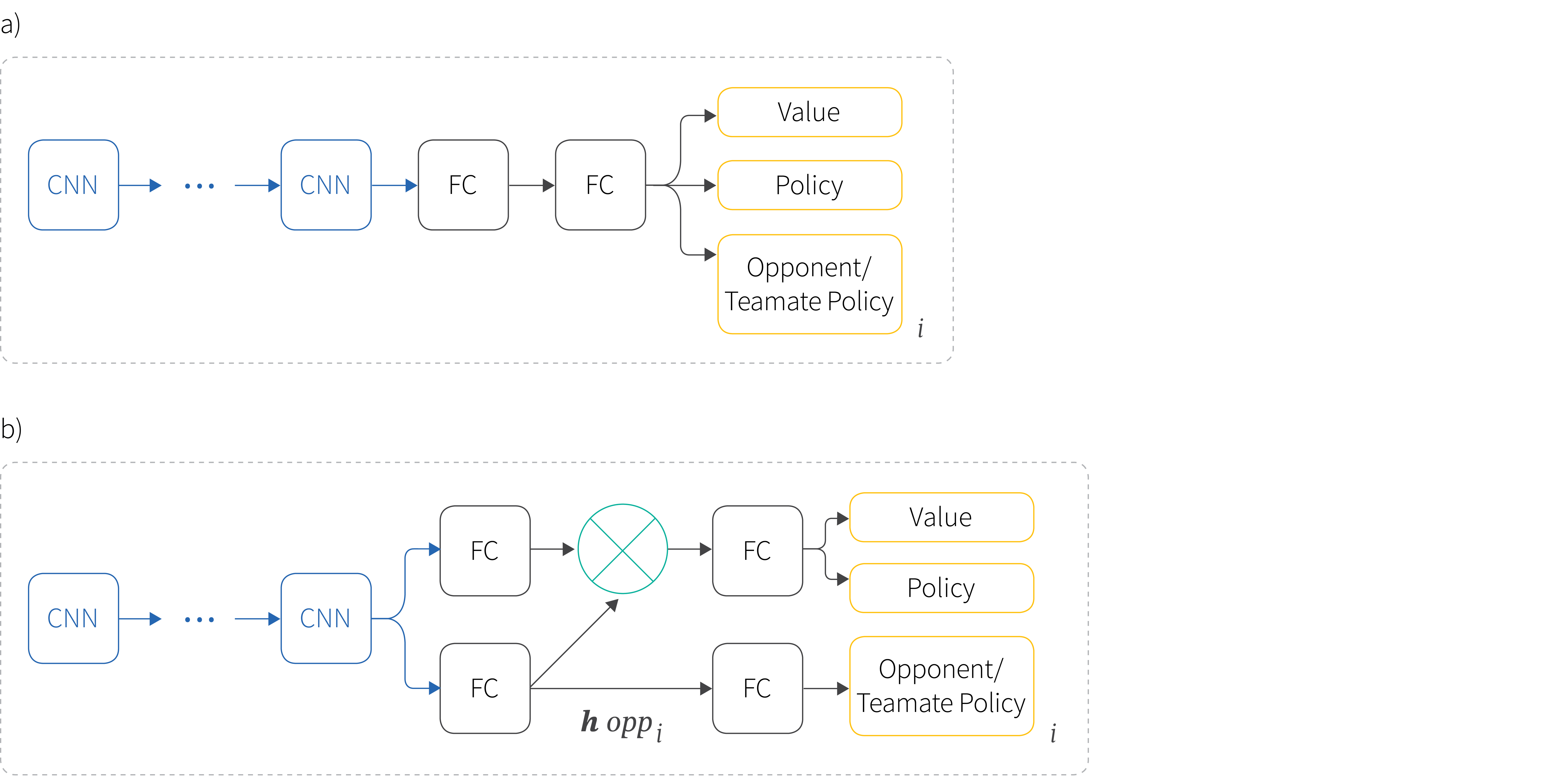
Figure 2. Agent modeling. a) Agent modeling by parameter sharing (AMS). The network shares a common representation for actor/critic computation and estimating the policies of other agents. b) Agent modeling with policy features (AMF): the network is divided in two sections, one learns opponent policies (bottom) and another learns value and policy of the agent (top). The opponent policy features, $\mathbf{h}_{opp}$, are used to condition the actor critic computation via an element-wise multiplication.
Agent modeling with policy features (AMF)
Policy features (Hong et al. 2018) are intermediate features from the latent space that is used to predict the opponent policy. The AMF framework exploits these features to improve the main reward prediction.
In this architecture, convolutional layers are shared, but the fully connected layers are divided in two sections (Figure 2b). The first is specialized for the actor and critic of the learning agent and the second for the opponent policies. The intermediate opponent policy features, $\mathbf{h}_{i}$ from the second path are used to condition (via an element-wise multiplication) the computation of the actor and critic. The loss function is similar to that for AMS.
Note that both AMS and AMF need to observe the opponent’s actions to generate ground truth and for the auxiliary loss function. This is a limitation, and further research is required to handle partially observable environments.
Task #3: Reward prediction
In the previous two sections, we considered auxiliary tasks that related to the structure of the learning (terminal prediction) and to other agents’ actions (agent modeling). In this section, we consider predicting the reward received at the next time-step — an idea that seems quite natural in the context of RL. More precisely, given state sequence $\{\mathbf{s}_{t-3}, \mathbf{s}_{t-2}, \mathbf{s}_{t-1}\}$, we aim to predict the reward $r_t$. Note that is similar to value learning with $\gamma=0$, so that the agent only cares about the immediate reward.
Jaderberg et al. (2017) formulated this task as multi-class classification with three classes: positive reward, negative reward, or zero. To mitigate data imbalance problems, the same number of samples with zero and non-zero rewards were provided during training.
In general, data imbalance is a disadvantage of reward prediction. This is particularly troublesome for hard-exploration problems with sparse rewards. For example, in the Pommerman game, an episode can last up to 800 timesteps, and the only non-zero reward is obtained at episode termination. Here, class-balancing would require many episodes, and this is in contradiction with the stated goal of using auxiliary tasks (i.e., to speed up learning).
Task #4: Depth prediction
Mirowski et al. (2016) studied auxiliary tasks in a navigation problem in which the agent needs to reach a goal in first-person 3D mazes from a random starting location. If the goal is reached, the agent is re-spawned to a new start location and must return to the goal. The 8 discrete actions permitted rotation and acceleration.
The agent sees RGB images as input. However, the authors speculated that depth information might supply valuable information about how to navigate the 3D environment. Thus, one of the auxiliary tasks is to predict depth, which can be cast as a regression or as a classification problem.
Mirowski et al. (2016) performed different experiments and we highlight two of these. In the first, they considered using the auxiliary task directly as input to the network, instead of just using it for computing the loss. In the second, they consider where to add the auxiliary task within the network. For example, the auxiliary task module can be set just after the convolutional layers, or after the convolutional and recurrent layers (Figure 3).

Figure 3. Depth prediction network. The depth auxiliary task prediction was evaluated after the convolutional layers (D2) or after the recurrent layers (D1). The input to the convolutional layers is the state at time t. The reward $r{t-1}$ on the previous timestep is an additional input to the first LSTM. The current velocity $v{t}$ of the agent and the agent’s action $a_{t-1}$ on the previous timestep are additional inputs to the second LSTM.
The results showed that:
- Using depth as input to the CNN (not shown in above Figure) resulted in worse performance than when predicting the depth.
- Treating depth estimation as classification (discretizing over 8 regions) outperformed casting it as regression.
- Placing the auxiliary task after the convolutional and recurrent networks obtained better results than moving it before the recurrent layers.
Task #5: Pixel control
The auxiliary tasks discussed so far have involved estimating various quantities. A control task actually tries to manipulate the environment in some way. Jaderberg et al. (2017) proposed pixel control auxiliary tasks. An auxiliary control task $c$ is defined by a reward function $r^{c}: \mathcal{S} \times \mathcal{A} \rightarrow \mathbb{R}$ where $\mathcal{S}$ is the space of possible states and $\mathcal{A}$ is the space of available actions. Given a base policy $\pi$, and auxiliary control task with policy $\pi^c$, the learning objective becomes:
\begin{equation}\mathcal{L}_{pc}= \mathbb{E}_{\pi}[R] + \lambda_{c} \mathbb{E}_{\pi^c}[R^{c}],\tag{6}\end{equation}
where $R^c$ is the return obtained from the auxiliary control task and $\lambda_{c}$ is a weight. As for previous auxiliary tasks, some parameters are shared with the main task.
The system used off-policy learning; the data was replayed from an experience buffer and the system was optimized using a n-step Q-learning loss:
\begin{equation} \mathcal{L}^c=(R_{t:t+n} + \gamma^n \max_{a’}\left[ Q^c(s’,a’,\boldsymbol\theta^{-})- Q^c(s,a,\boldsymbol\theta))^2\right]\tag{7}\end{equation}
where $\boldsymbol\theta$ and $\boldsymbol\theta^{-}$ refers are the current and previous parameters, respectively.
Jaderberg et al. (2017) noted that changes in the perceptual stream are important since they generally correspond to important events in an environment. Thus, the agent learns a policy for maximally changing the pixels in each cell of an $n \times n$ non-overlapping grid superimposed on the input image. The immediate reward in each cell was defined as the average absolute difference from the previous frame. Results show that these types of auxiliary task can significantly improve learning.
Challenges
In this section we consider some unresolved challenges associated with using auxiliary tasks in deep RL.
Defining a good auxiliary task
We have seen that adding an auxiliary task is relatively simple. However, the first and most important challenge is to define a good auxiliary task. Exactly how to do this remains an open question.
As a step towards this, Du et al. (2018) devised a method to detect when a given auxiliary task might be useful. Their approach uses the intuition that an algorithm should take advantage of the auxiliary task when it is helpful for the main task and block it otherwise.
Their proposal has two parts. First, they determine whether the auxiliary task and the main task are related. Second, they modulate how useful the auxiliary task is with respect to the main task using a weight. In particular, they propose to detect when an auxiliary loss $\mathcal{L}_{aux}$ is helpful to the main loss $\mathcal{L}_{main}$ by using the cosine similarity between gradients of the two losses:
Algorithm 1: Use of auxiliary task by gradient similarity
if $\cos[\nabla_{\theta}\mathcal{L}_{main},\nabla_{\theta} \mathcal{L}_{aux}]\ge 0$ then
| Update $\theta$ using $\nabla_{\theta}\mathcal{L}_{main} +\nabla_{\theta} \mathcal{L}_{aux}$
else
| Update $\theta$ using $\nabla_{\theta}\mathcal{L}_{main}$
end
The goal of this algorithm is to avoid adding an auxiliary loss that impedes learning progress for the main task. This is sensible, but would ideally be augmented by a better theoretical understanding of the benefits (Bellemare et al. 2019).
Choosing the auxiliary weight
The auxiliary task is always accompanied by a weight but it’s not obvious how to choose its value. Ideally, this weight should give enough importance to the auxiliary task to drive the representation learning but also one needs to be careful not to ignore the main task.
Weights need not be fixed, and can vary over time. Hernandez-Leal et al. (2019) compared five different weight parameterizations for the agent modeling task. In some the weight was fixed and in others it decayed. Figure 4 shows that, in the same environment, this choice directly affects the performance.
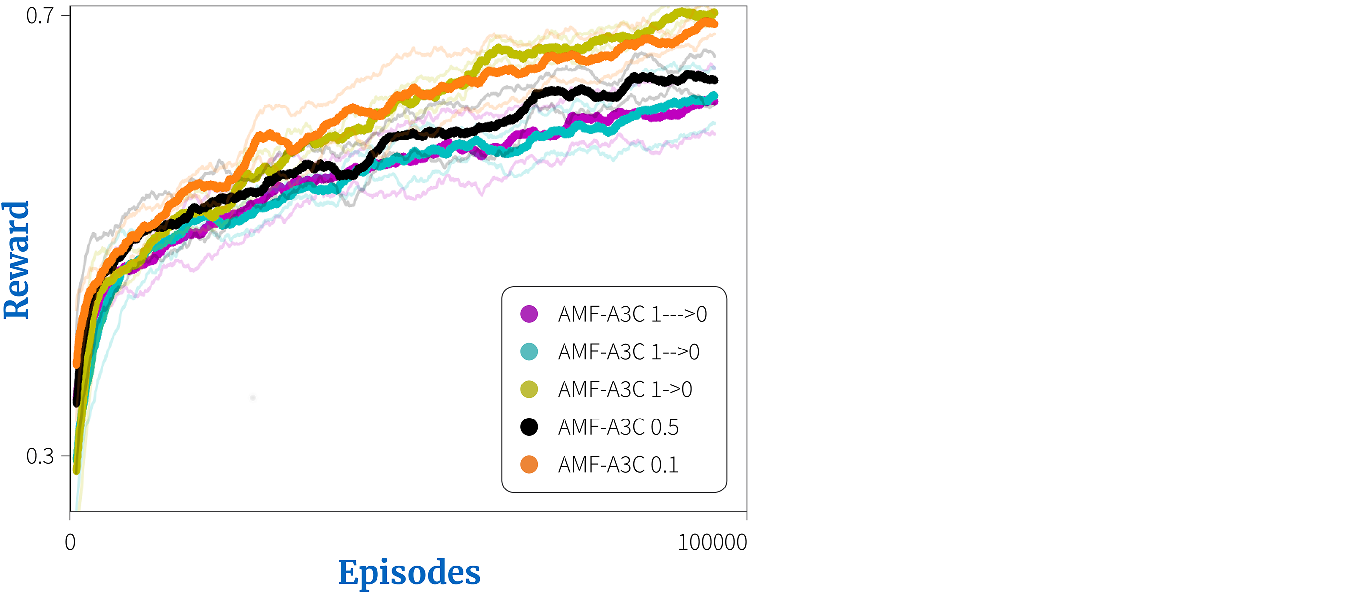
Figure 4. Choosing the auxiliary weight. Hernandez-Leal et al. (2019) investigated different weighting schemes for their agent modeling task. They considered gradually decaying the weight at three different speeds ($1—>0$ begins with a weight of 1.0 and has an exponential decay rate of 0.99999, $1–>0$ corresponds to 0.9999, and $1->0$ corresponds to 0.999). There were also two fixed weight values (0.5 and 0.1). Different approaches lead to quite different performance.
It also appears that the optimal auxiliary weight is dependent on the domain. For the tasks discussed in this post:
- Terminal prediction used a weight of 0.5 (Kartal et al. 2019).
- Reward prediction used a weight of 1.0 (Jaderberg et al. 2017).
- Auxiliary control varied between 0.0001 and 0.01 (Jaderberg et al. 2017).
- Depth prediction chose from the set {1, 3.33, 10} (Mirowski et al. 2016).
Benefits
In the last part of this article we discuss the two major benefits of using auxiliary tasks: improving performance and increasing robustness.
Improved performance
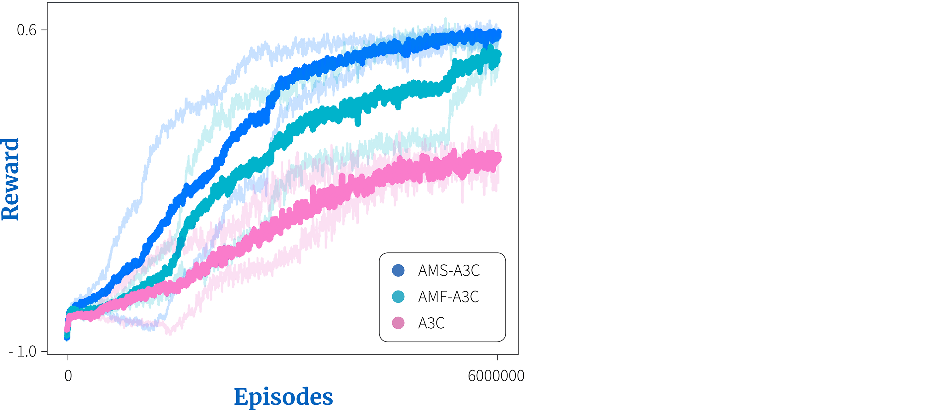
Figure 5. Results for the agent modeling auxiliary task from Hernandez-Leal et al. (2019). Both agent modelling with parameter sharing (AMS-A3C) and agent modelling with policy features (AMF-A3C), improve performance over vanilla A3C on the Pommerman domain.
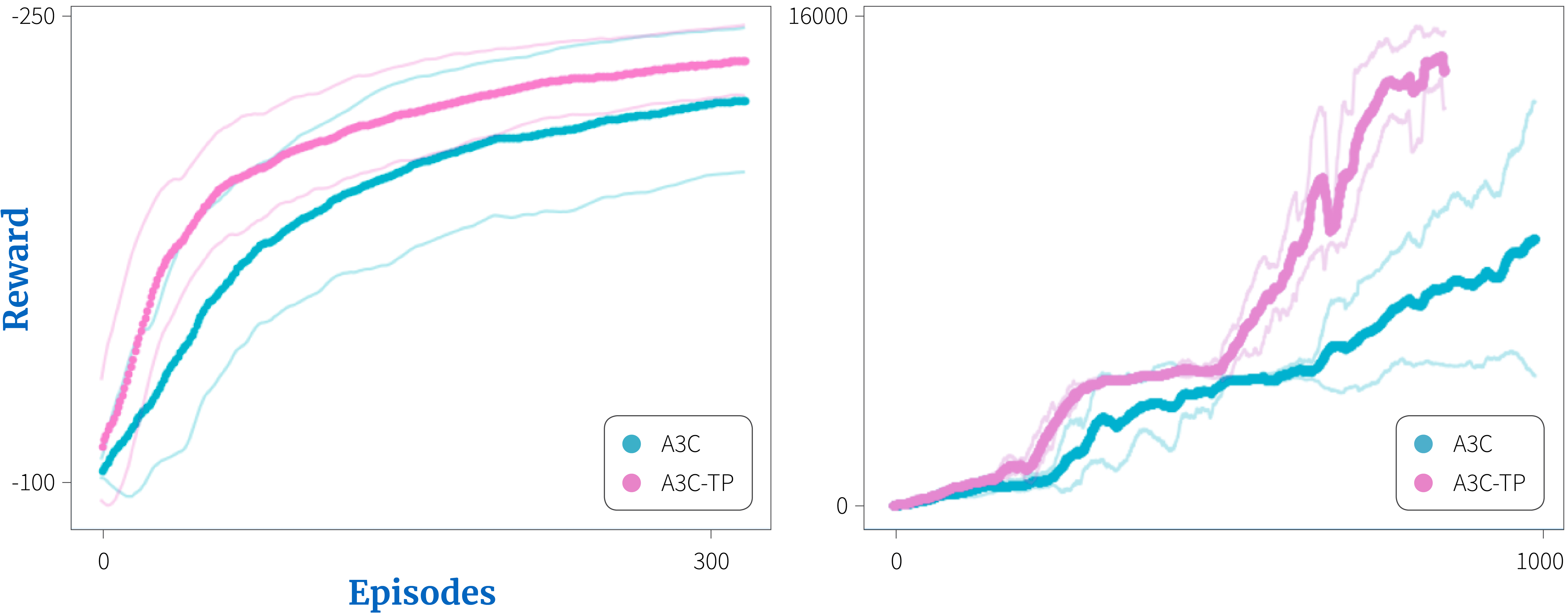
Figure 6. Terminal prediction results from Kartal et al. (2019). a) Terminal prediction auxiliary task on the Q*bert Atari game. b) Terminal prediction auxiliary task on the Bipedal Walker domain.
The main benefit of auxiliary tasks is to drive representation learning and hence improve the agent’s performance; the system learns faster and achieves better performance in terms of rewards with an appropriate auxiliary task.
For example, when auxiliary tasks where added to A3C agents, scores improved in domains such as Pommerman (Figure 5), Q*bert (Figure 6a) and the Bipedal walker (Figure 6b). Similar benefits of auxiliary tasks have been shown in Q-learning style algorithms (Lample & Chaplot 2017; Fedus et al. 2019).
Increased robustness
The second benefit is related to robustness, and we believe this has been somewhat under-appreciated. One problem with deep RL is the high variance over different runs. This can even happen in the same experiment while just varying the random seed (Henderson et al. 2018). This is a major complication because algorithms sometimes diverge (i.e., they fail to learn) and thus we prefer robust algorithms that can learn under a variety of different values for their parameters.
Auxiliary tasks have been shown to improve robustness of the learning process. In the UNREAL work (Jaderberg et al. 2017), the authors varied two hyperparameters, entropy cost and learning rate, and kept track of the final performance while adding different auxiliary tasks. The results showed that adding auxiliary tasks increased performance over a variety of hyperparameter values (Figure 7).
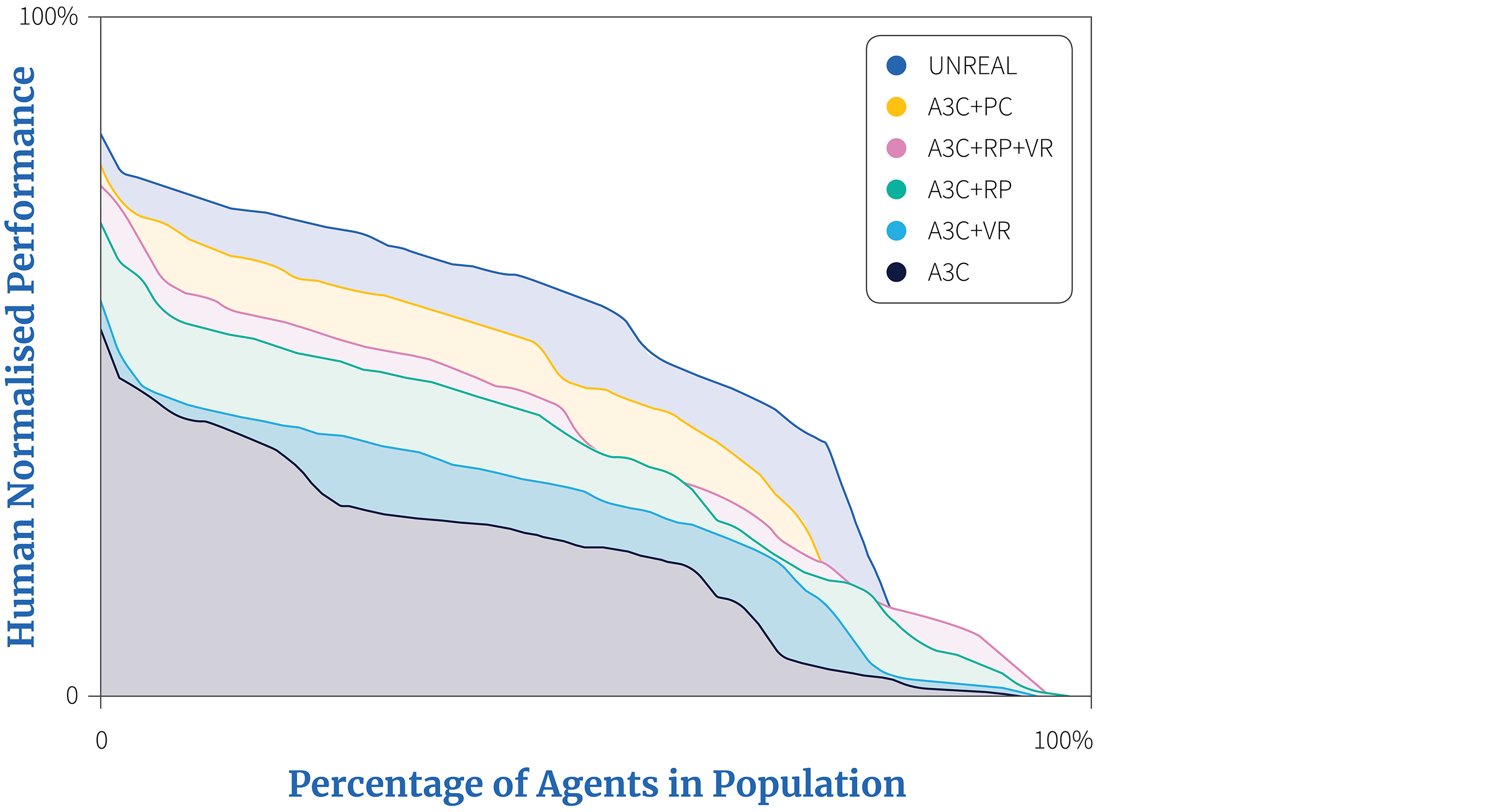
Figure 7. This graphs shows the final human-normalised score in a hyperparameter sweep, sorted by score (and thus higher curves are better). The vanilla A3C algorithm is compared to variants that have pixel control (PC), reward prediction (RP), and/or value function replay (VR), where the UNREAL agent uses all three auxiliary tasks. UNREAL increases the robustness with respect to the learning rate and entropy hyperparameters.
Conclusions
In this tutorial we reviewed auxiliary tasks in the context of deep reinforcement learning and we presented examples from a variety of domains. Auxiliary tasks been used to accelerate and provide robustness to the learning process. However, there are still open questions and challenges such as defining what constitutes a good auxiliary task and forming a better theoretical understanding of how they contribute.
1Note that the RL agent does not have access to the time stamp or a memory, so it must predict its time relative to the terminal state afresh at each time step.
Work with Us!
Impressed by the work of the team? RBC Borealis is looking to hire for various roles across different teams. Visit our career page now and discover opportunities to join similar impactful projects!
Careers at RBC Borealis