
The goal of the variational autoencoder (VAE) is to learn a probability distribution $Pr(\mathbf{x})$ over a multi-dimensional variable $\mathbf{x}$. There are two main reasons for modelling distributions. First, we might want to draw samples (generate) from the distribution to create new plausible values of $\mathbf{x}$. Second, we might want to measure the likelihood that a new vector $\mathbf{x}^{*}$ was created by this probability distribution. In fact, it turns out that the variational autoencoder is well-suited to the former task but not for the latter.
It is common to talk about the variational autoencoder as if it is the model of $Pr(\mathbf{x})$. However, this is misleading; the variational autoencoder is a neural architecture that is designed to help learn the model for $Pr(\mathbf{x})$. The final model contains neither the ‘variational’ nor the ‘autoencoder’ parts and is better described as a non-linear latent variable model.
We’ll start this tutorial by discussing latent variable models in general and then the specific case of the non-linear latent variable model. We’ll see that maximum likelihood learning of this model is not straightforward, but we can define a lower bound on the likelihood. We then show how the autoencoder architecture can approximate this bound using a Monte Carlo (sampling) method. To maximize the bound, we need to compute derivatives, but unfortunately, it’s not possible to compute the derivative of the sampling component. We’ll show how to side-step this problem using the reparameterization trick. Finally, we’ll discuss extensions of the VAE and some of its drawbacks.
Latent variable models
Latent variable models take an indirect approach to describing a probability distribution $Pr(\mathbf{x})$ over a multi-dimensional variable $\mathbf{x}$. Instead of directly writing the expression for $Pr(\mathbf{x})$ they model a joint distribution $Pr(\mathbf{x}, \mathbf{h})$ of the data $\mathbf{x}$ and an unobserved latent (or hidden) variable $\mathbf{h}$. They then describe the probability of $Pr(\mathbf{x})$ as a marginalization of this joint probability so that
\begin{equation} Pr(\mathbf{x}) = \int Pr(\mathbf{x}, \mathbf{h}) d\mathbf{h}.\tag{1}\end{equation}
Typically we describe the joint probability $Pr(\mathbf{x}, \mathbf{h})$ as the product of the likelihood $Pr(\mathbf{x}|\mathbf{h})$ and the prior $Pr(\mathbf{h})$, so that the model becomes
\begin{equation} Pr(\mathbf{x}) = \int Pr(\mathbf{x}| \mathbf{h}) Pr(\mathbf{h}) d\mathbf{h}.\tag{2}\end{equation}
It is reasonable to question why we should take this indirect approach to describing $Pr(\mathbf{x})$. The answer is that relatively simple expressions for $Pr(\mathbf{x}| \mathbf{h})$ and $Pr(\mathbf{h})$ can describe a very complex distribution for $Pr(\mathbf{x})$.
Example: mixture of Gaussians
A well known latent variable model is the mixture of Gaussians. Here the latent variable $h$ is discrete and the prior $Pr(h)$ is a discrete distribution with one probability $\lambda_{k}$ for each of the $K$ component Gaussians. The likelihood $Pr(\mathbf{x}|h)$ is a Gaussian with a mean $\boldsymbol\mu_{k}$ and covariance $\boldsymbol\Sigma_{k}$ that depends on the value $k$ of the latent variable $h$:
\begin{eqnarray} Pr(h=k) &=& \lambda_{k}\nonumber \\ Pr(\mathbf{x} |h = k) &=& \mbox{Norm}_{\mathbf{x}}[\boldsymbol\mu_{k},\boldsymbol\Sigma_{k}].\label{eq:mog_like_prior}\tag{3}\end{eqnarray}
where $\mbox{Norm}_{\mathbf{x}}[\boldsymbol\mu, \boldsymbol\Sigma]$ represents a multivariate probability distribution over $\mathbf{x}$ with mean $\boldsymbol\mu$ and covariance $\boldsymbol\Sigma$.
As in equation 2, the likelihood $Pr(x)$ is given by the marginalization over the latent variable $h$. In this case, this is a sum as the latent variable is discrete:
\begin{eqnarray} Pr(\mathbf{x}) &=& \sum_{k=1}^{K} Pr(\mathbf{x}, h=k) \nonumber \\ &=& \sum_{k=1}^{K} Pr(\mathbf{x}| h=k) Pr(h=k)\nonumber \\ &=& \sum_{k=1}^{K} \lambda_{k} \mbox{Norm}_{\mathbf{x}}[\boldsymbol\mu_{k},\boldsymbol\Sigma_{k}]. \tag{4}\end{eqnarray}
This is illustrated in figure 1. From the simple expressions for the likelihood and prior in equation 3, we can describe a complex multi-modal probability distribution.
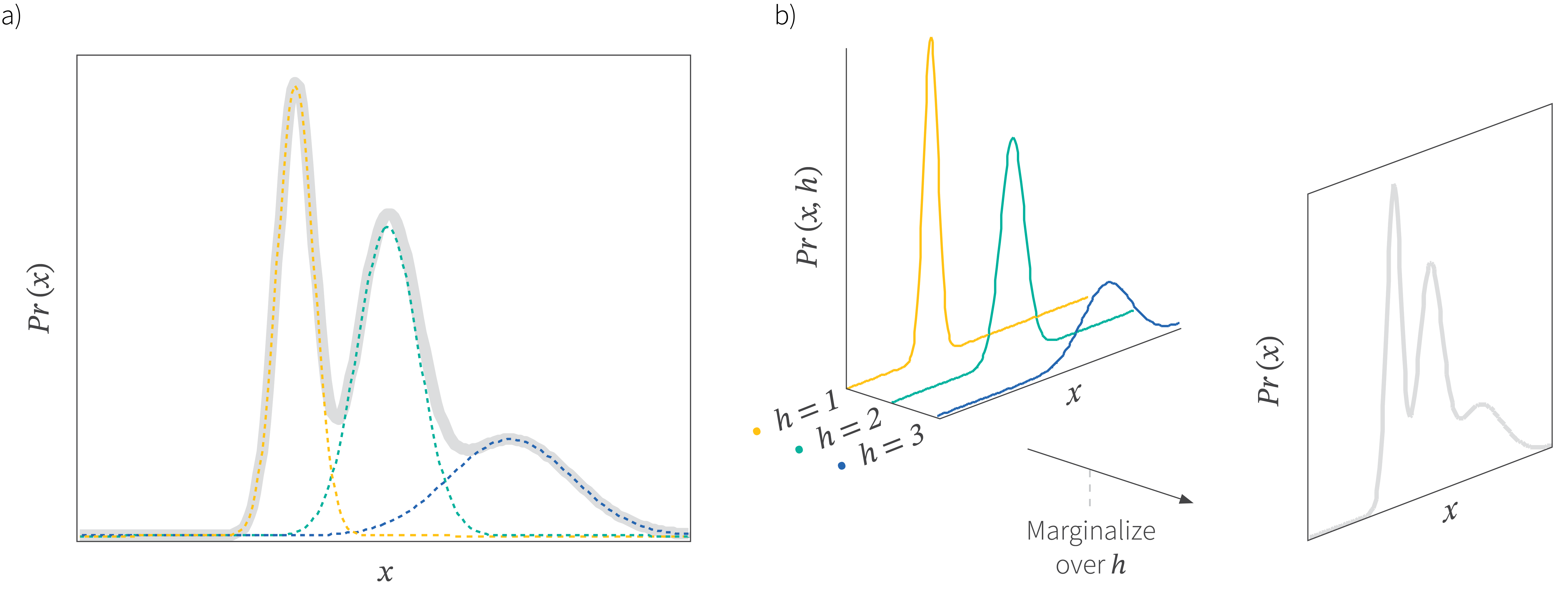
Figure 1. Mixture of Gaussians. a) A mixture of Gaussians creates a complex probability distribution as a weighted sum of several simpler Gaussian components. b) The mixture of Gaussians model can be seen as a marginalization of the joint density $Pr(x,h)$ between the continuous observed data $x$ and a discrete latent or hidden variable $h$.
Non-linear latent variable model
Now let’s consider the non-linear latent variable model, which is what the VAE actually learns. This differs from the mixture of Gaussians in two main ways. First, the latent variable $\mathbf{h}$ is continuous rather than discrete and has a standard normal prior (i.e., one with mean zero and identity covariance). Second, the likelihood is a normal distribution as before, but the variance is constant and spherical. The mean is a non-linear function $\mathbf{f}[\mathbf{h},\bullet]$ of the hidden variable $\mathbf{h}$ and this gives rise to the name. The prior and likelihood terms are:
\begin{eqnarray} Pr(\mathbf{h}) &=& \mbox{Norm}_{\mathbf{h}}[\mathbf{0},\mathbf{I}]\nonumber \\ Pr(\mathbf{x} |\mathbf{h},\boldsymbol\phi) &=& \mbox{Norm}_{\mathbf{x}}[\mathbf{f}[\mathbf{h},\boldsymbol\phi],\sigma^{2}\mathbf{I}], \tag{5}\end{eqnarray}
where the function $\mathbf{f}[\mathbf{h},\boldsymbol\phi]$ is a deep neural network with parameters $\boldsymbol\phi$. This model is illustrated in figure 2.
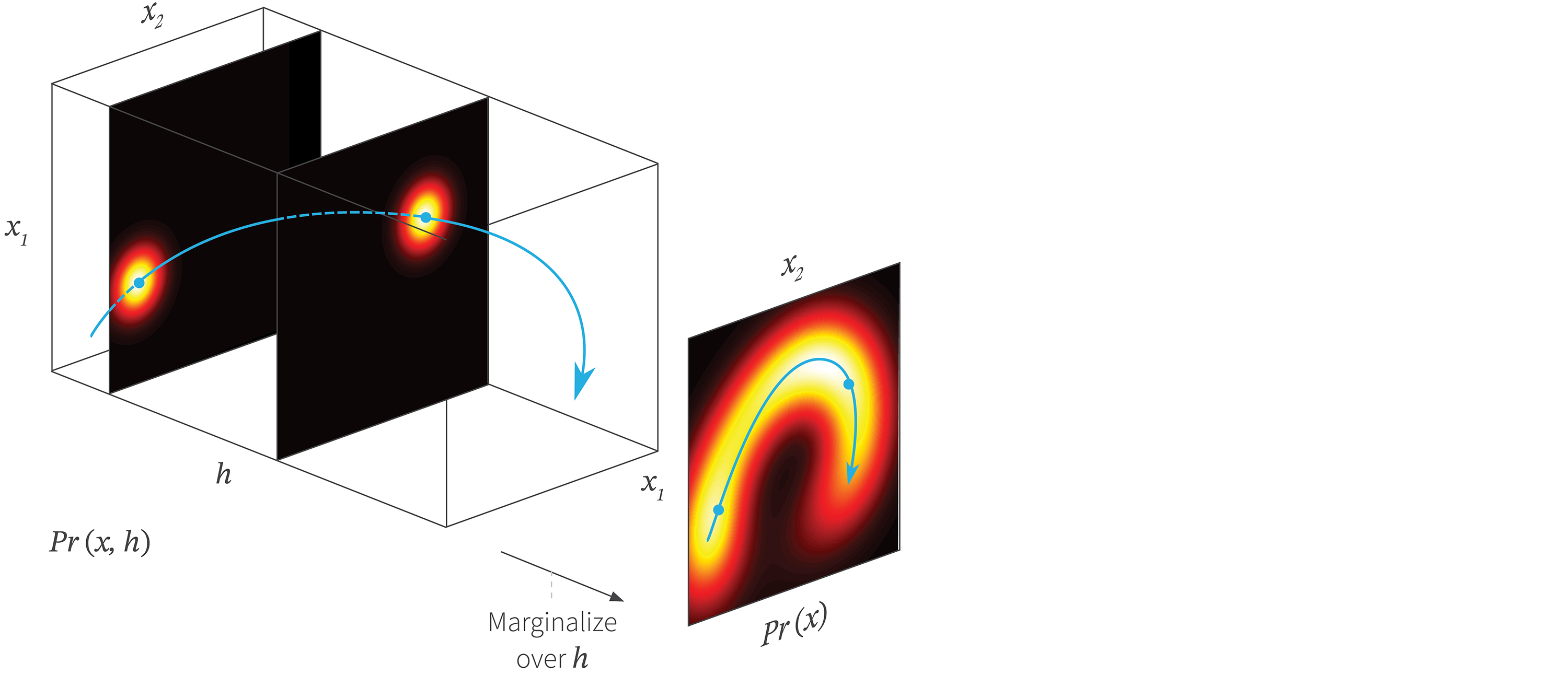
Figure 2. Non-linear latent variable model. A complex 2D density $Pr(\mathbf{x})$ (right) is created as a the marginalization of the joint distribution $Pr(\mathbf{x},h)$ (left) over the latent or hidden variable $h$; to create the 2D density we integrate over the 3D volume along the dimension $h$. For each value of $h$ the distribution over $\mathbf{x}$ is a spherical Gaussian with a mean that depends on $\mathbf{h}$ (two slices shown). The mean is a non-linear function $\mathbf{f}[h,\boldsymbol\phi]$ (blue curve) of the hidden variable and the shape of this function depends on parameters $\boldsymbol\phi$. When we sum all of these spherical Gaussians we get the complex data density $Pr(\mathbf{x})$.
The model can be viewed as an infinite mixture of spherical Gaussians with different means; as before, we build a complex distribution by weighting and summing these Gaussians in the marginalization process. In the next three sections we consider three operations that we might want to perform with this model: computing the posterior distribution, sampling, and evaluating the likelihood.
Computing the posterior
The likelihood $Pr(\mathbf{x} |\mathbf{h},\boldsymbol\phi)$ tells us how to compute the distribution over the observed data $\mathbf{x}$ given hidden variable $\mathbf{h}$. We might however want to move in the other direction; given an observed data example $\mathbf{x}$ we might wish to understand what possible values of the hidden variable $\mathbf{h}$ were responsible for it (figure 3). This information is encompassed in the posterior distribution $Pr(\mathbf{h}|\mathbf{x})$. In principle, we can compute this using Bayes’s rule
\begin{eqnarray} Pr(\mathbf{h}|\mathbf{x}) = \frac{Pr(\mathbf{x}|\mathbf{h})Pr(\mathbf{h})}{Pr(\mathbf{x})}. \tag{6}\end{eqnarray}
However, in practice, there is no closed form expression for the left hand side of this equation. In fact, as we shall see shortly, we cannot evaluate the denominator $Pr(\mathbf{x})$ and so we can’t even compute the numerical value of the posterior for a given pair $\mathbf{h}$ and $\mathbf{x}$.
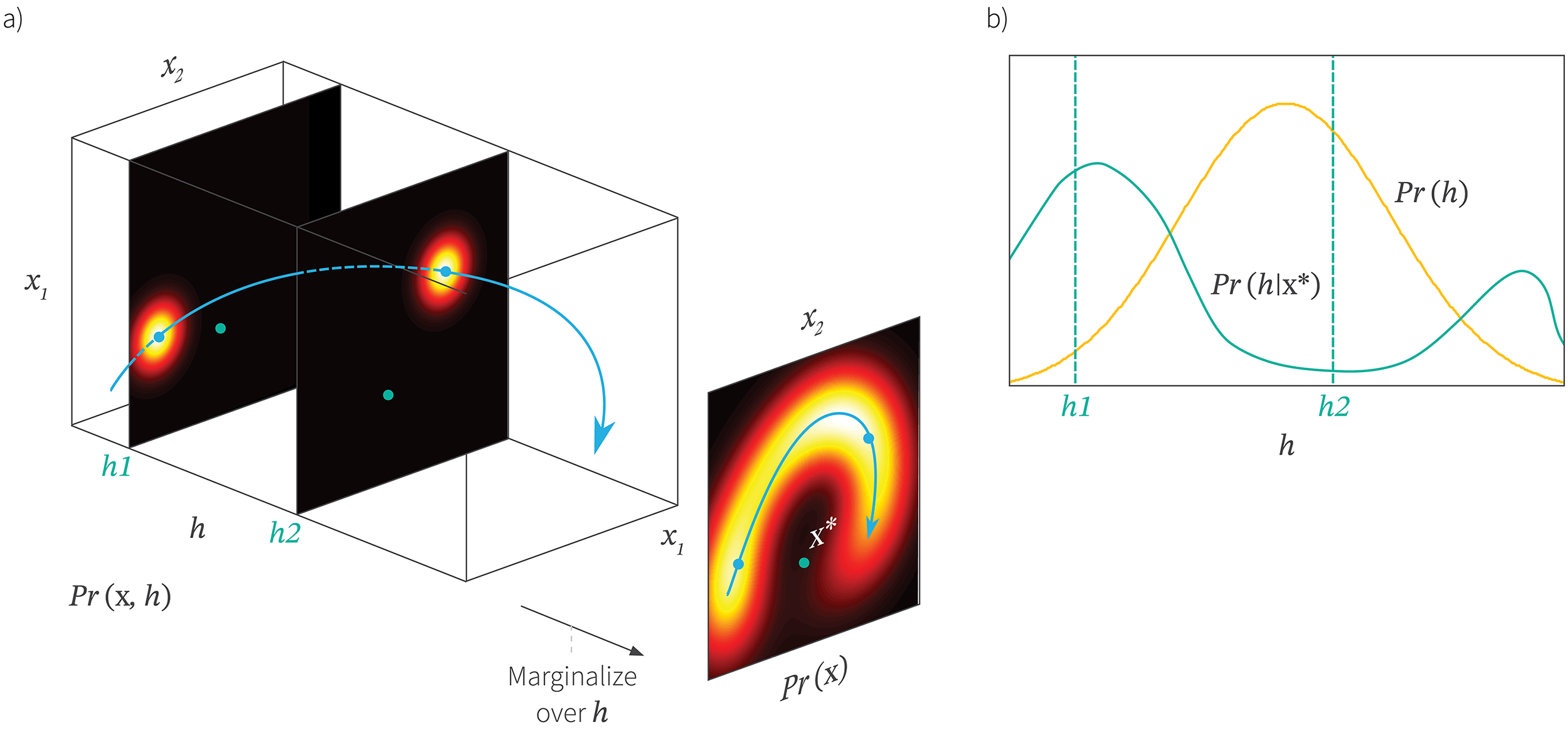
Figure 3. Posterior distribution over latent variable. a) The posterior distribution $Pr(h|\mathbf{x}^{*})$ is the distribution over possible values of the latent variable $h$ that could be responsible for a new data point $\mathbf{x}^{*}$ (green point). We compute this via Bayes’ rule $Pr(h|\mathbf{x}^{*})\propto Pr(\mathbf{x}^{*}|h)Pr(h)$. We compute the first term on the rhs (the likelihood) by assessing the probability of $\mathbf{x}^{*}$ against the symmetric Gaussian associated with each value of $h$. Here you can see that it was more likely to have been created from $h_{1}$ than $h_{2}$. b) The second term that influences the posterior is the prior probability $Pr(h)$ over the hidden variable (yellow curve). Combining these two factors together and normalizing so the distribution sums to one gives us the posterior $Pr(h|\mathbf{x}^{*})$. In general, computing this distribution is intractable; it has no convenient parametric form.
Generation
Although computing the posterior is intractable, it is easy to generate a new sample $\mathbf{x}^{*}$ from this model using ancestral sampling; we draw $\mathbf{h}^{*}$ from the prior $Pr(\mathbf{h})$, pass this through the network $f[\mathbf{h}^{*},\boldsymbol\phi]$ to compute the mean of the likelihood $Pr(\mathbf{x}|\mathbf{h})$ and then draw $\mathbf{x}$ from this distribution. Both the prior and the likelihood are normal distributions and so sampling from them in each step is easy. This process is illustrated in figure 4.

Figure 4. Generation from non-linear latent variable model. a) We draw a sample $h^{*}$ from the prior probability $Pr(h)$ over the hidden variable. b) A sample $\mathbf{x}^{*}$ is then drawn from $Pr(\mathbf{x}|h^{*}$). This distribution is a spherical Gaussian with a mean that is a non-linear function of $h^{*}$ and a fixed spherical covariance. c) If we repeat this process a very large number of times, we recover the density $Pr(\mathbf{x})$.
Evaluating Likelihood
Finally, let’s consider evaluating the likelihood of a data example $\mathbf{x}$ under the model. As before, the likelihood is given by:
\begin{eqnarray} Pr(\mathbf{x}) &=& \int Pr(\mathbf{x}, \mathbf{h}|\boldsymbol\phi) d\mathbf{h} \nonumber \\ &=& \int Pr(\mathbf{x}| \mathbf{h},\boldsymbol\phi) Pr(\mathbf{h})d\mathbf{h}\nonumber \\ &=& \int \mbox{Norm}_{\mathbf{x}}[\mathbf{f}[\mathbf{h},\boldsymbol\phi],\sigma^{2}\mathbf{I}]\mbox{Norm}_{\mathbf{h}}[\mathbf{0},\mathbf{I}]d\mathbf{h}. \tag{7}\end{eqnarray}
Unfortunately, there is no closed form for this integral, so we cannot easily compute the probability for a given example $\mathbf{x}$. This is a major problem for two reasons. First, evaluating the probability $Pr(\mathbf{x})$ was of the main reasons for modelling the probability distribution in the first place. Second, to learn the model, we maximize the log likelihood, which is obviously going to be hard if we cannot compute it. In the next section we’ll introduce a lower bound on the log likelihood which can be computed and which we can use to learn the model.
Evidence lower bound (ELBO)
During learning we are given training data $\{\mathbf{x}_{i}\}_{i=1}^{I}$ and want to maximize the log likelihood of the model with respect to the parameters $\boldsymbol\phi$. For simplicity we’ll assume that the variance term $\sigma^2$ in the likelihood expression is known and just concentrate on learning $\boldsymbol\phi$:
\begin{eqnarray} \hat{\boldsymbol\phi} &=& argmax_{\boldsymbol\phi} \left[\sum_{i=1}^{I}\log\left[Pr(\mathbf{x}_{i}|\boldsymbol\phi) \right]\right] \nonumber \\ &=& argmax_{\boldsymbol\phi} \left[\sum_{i=1}^{I}\log\left[\int Pr(\mathbf{x}_{i}, \mathbf{h}_{i}|\boldsymbol\phi) d\mathbf{h}_{i}\right]\right].\label{eq:log_like} \tag{8}\end{eqnarray}
As we noted above, we cannot write a closed form expression for the integral and so we can’t just build a network to compute this and let Tensorflow or PyTorch optimize it.
To make some progress we define a lower bound on the log likelihood. This is a function that is always less than or equal to the log likelihood for a given value of $\boldsymbol\phi$ and will also depend on some other parameters $\boldsymbol\theta$. Eventually we will build a network to compute this lower bound and optimize it. To define this lower bound, we need to use Jensen’s inequality which we quickly review in the next section.
Jensen’s inequality
Jensen’s inequality concerns what happens when we pass values through a concave function $g[\bullet]$. Specifically, it says that if we compute the expectation (mean) of these values and pass this mean through the function, the results will be greater than if we pass the values themselves through the function and then compute the expectation of the results. In mathematical terms:
\begin{equation} g[\mathbf{E}[y]] \geq \mathbf{E}[g[y]], \tag{9}\end{equation}
for any concave function $g[\bullet]$. Some intuition as to why this is true is given in figure 5. In our case, the concave function in question is the logarithm so we have:
\begin{equation} \log[\mathbf{E}[y]]\geq\mathbf{E}[\log[y]], \tag{10}\end{equation}
or writing out the expression for expectation in full we have:
\begin{equation} \log\left[\int Pr(y) y dy\right]\geq \int Pr(y)\log[y]dy. \tag{11}\end{equation}
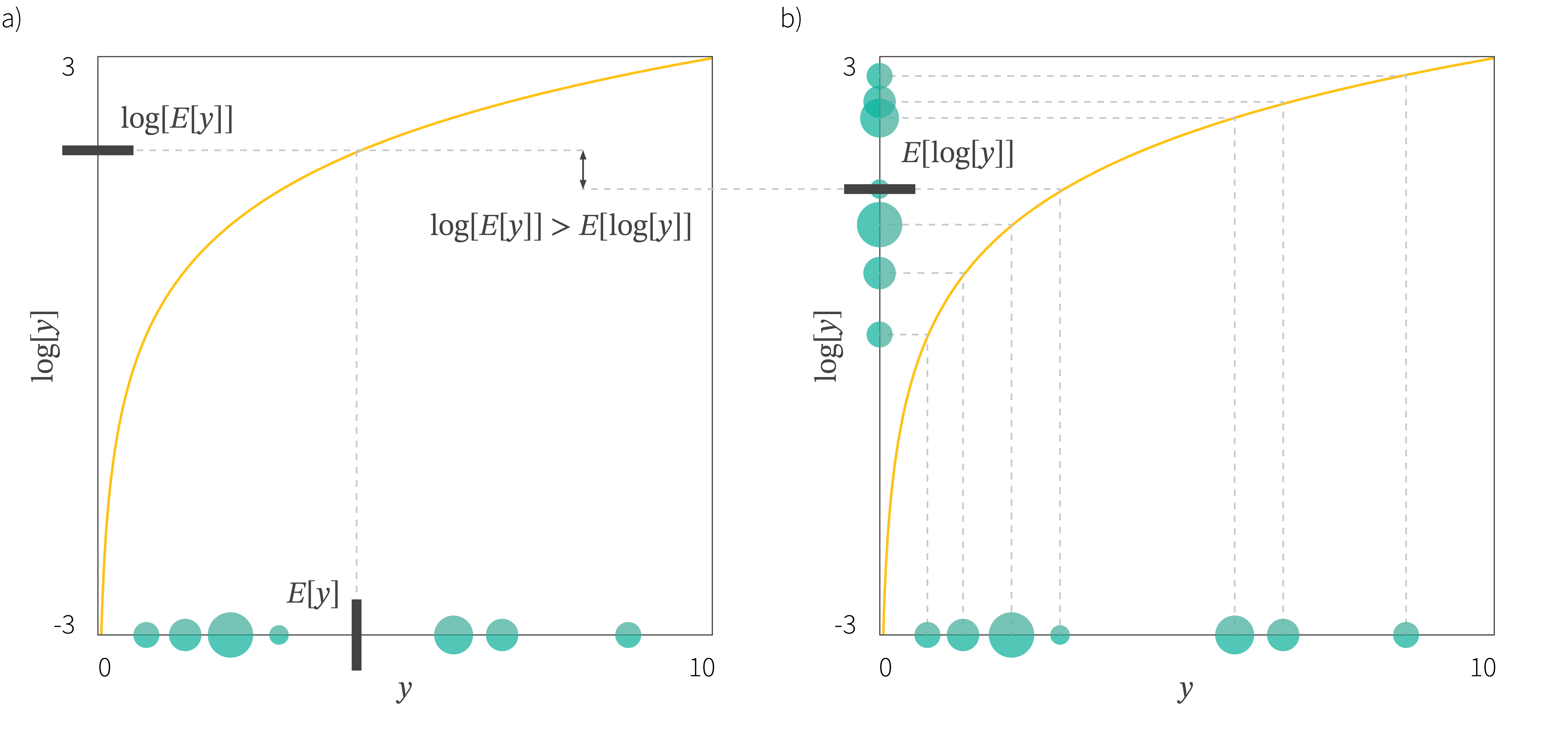
Figure 5. Jensen’s inequality. The logarithm (yellow curve) is a concave function because you can draw a straight line between any two points on the curve and this line will always lie underneath the curve. Consider a probability distribution on $y$ (here represented by weighted samples in green). Jensen’s inequality says that for a concave function when we compute the expectation of the distribution and pass it through the function, the result is always greater than or equal to passing the individual values $y$ through the function and then computing the expectation. In the case of the logarithm we have $\log[\mathbf{E}[y]] \geq \mathbf{E}[\log[y]]$. The left hand side of the figure corresponds to the left hand side of this inequality and the right hand side of the figure to the right hand side of the inequality. An intuition for Jensen’s inequality is as follows: the concave function relatively spreads out the low values of $y$ and compresses the high values, so the average is less when we pass $y$ through the function first.
Deriving the bound
We will now use Jensen’s inequality to derive the lower bound for the log likelihood. We start by multiplying and dividing the log likelihood by an arbitrary probability distribution $q(\mathbf{h})$ over the hidden variables
\begin{eqnarray}\log[Pr(\mathbf{x}|\boldsymbol\phi)] &=& \log\left[\int Pr(\mathbf{x},\mathbf{h}|\boldsymbol\phi)d\mathbf{h} \tag{12} \right] \\&=& \log\left[\int q(\mathbf{h}) \frac{ Pr(\mathbf{x},\mathbf{h}|\boldsymbol\phi)}{q(\mathbf{h})}d\mathbf{h} \tag{13} \right],\end{eqnarray}
We then use Jensen’s inequality for the logarithm (equation 11) to find a lower bound:
\begin{eqnarray}\log\left[\int q(\mathbf{h}) \frac{ Pr(\mathbf{x},\mathbf{h}|\boldsymbol\phi)}{q(\mathbf{h})}d\mathbf{h} \right]&\geq& \int q(\mathbf{h}) \log\left[\frac{ Pr(\mathbf{x},\mathbf{h}|\boldsymbol\phi)}{q(\mathbf{h})} \right]d\mathbf{h}, \tag{14}\end{eqnarray}
where the term on the right hand side is known as the evidence lower bound or ELBO. It gets this name because the term $Pr(\mathbf{x}|\boldsymbol\phi)$ is known as the evidence when viewed in the context of Bayes’ rule (equation 6).
In practice, the distribution $q(\mathbf{h})$ will have some parameters $\boldsymbol\theta$ as well and so the ELBO can be written as:
\begin{equation}\mbox{ELBO}[\boldsymbol\theta, \boldsymbol\phi] = \int q(\mathbf{h}|\boldsymbol\theta) \log\left[\frac{ Pr(\mathbf{x},\mathbf{h}|\boldsymbol\phi)}{q(\mathbf{h}|\boldsymbol\theta)} \right]d\mathbf{h}. \tag{15}\end{equation}
To learn the non-linear latent variable model, we’ll maximize this quantity as a function of both $\boldsymbol\phi$ and $\boldsymbol\theta$. The neural architecture that computes this quantity (and hence is used to optimize it) is the variational autoencoder. Before we introduce that, we first consider some of the properties of the ELBO.
ELBO properties
When first encountered, the ELBO can be a somewhat mysterious object. In this section we’ll provide some intuition about its properties. Consider that the original log likelihood of the data is a function of the parameters $\boldsymbol\phi$ and we want to find its maximum. For any fixed $\boldsymbol\theta$, the ELBO is still a function of the parameters, but one that must lie below the original likelihood function. When we change $\boldsymbol\theta$ we modify this function and depending on our choice, it may move closer or further from the log likelihood. When we change $\boldsymbol\phi$ we move along this function. These perturbations are illustrated in figure 6.
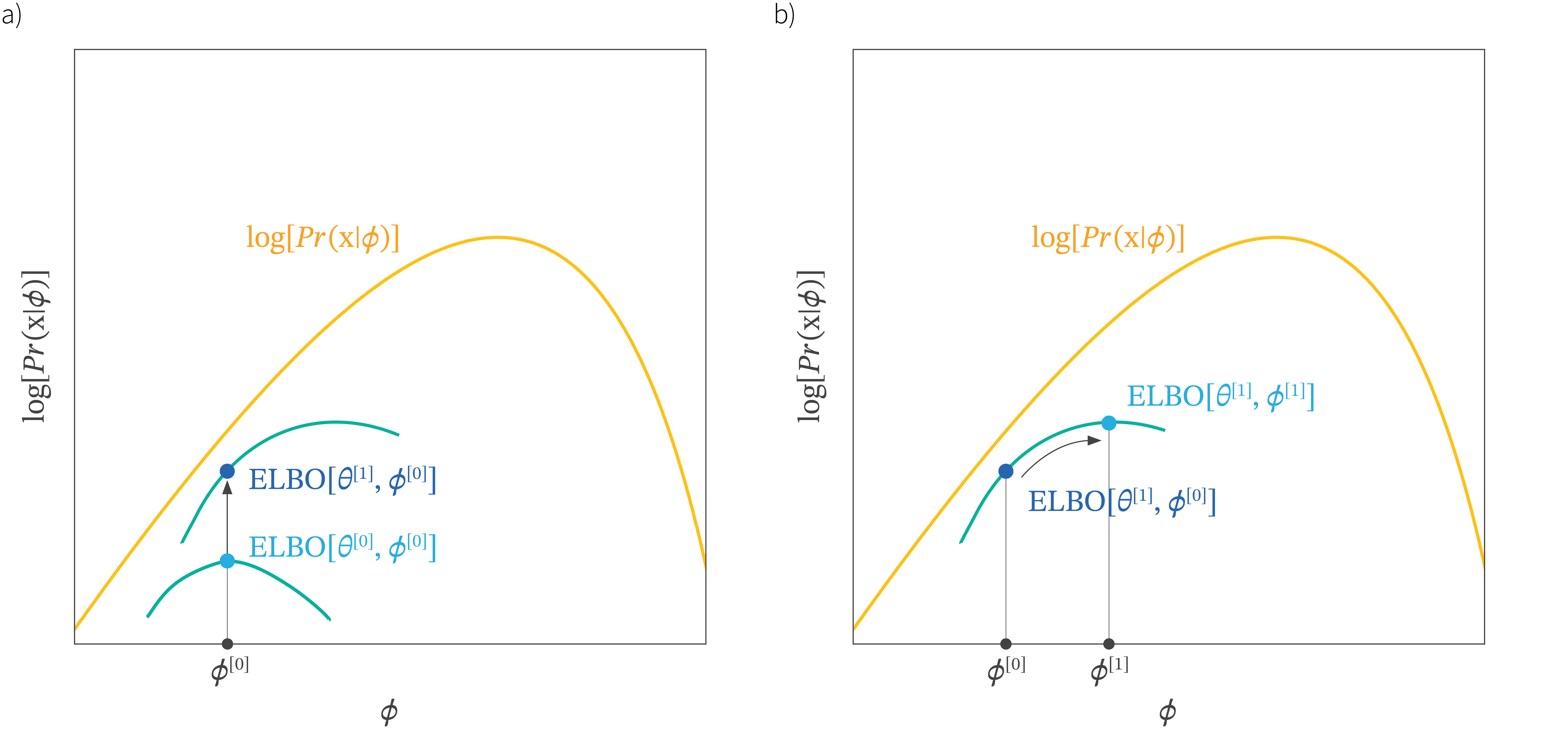
Figure 6. The evidence lower bound (ELBO). Our goal is to maximize the log likelihood $\log[Pr(\mathbf{x}|\boldsymbol\phi)]$ (yellow curve) with respect to the parameters $\boldsymbol\phi$. a) The ELBO is a function that lies everywhere below the log likelihood. It is a function of both $\boldsymbol\phi$ and a second set of parameters $\boldsymbol\theta$. For fixed $\boldsymbol\theta$ we get a function of $\boldsymbol\phi$ that is lies below the log likelihood (two green curves for different values of $\boldsymbol\theta$). Consequently, we can get closer to the maximum log likelihood by either a) improving the bound with respect to the new parameters $\boldsymbol\theta$ or b) moving along the current bound with respect to the original parameters $\boldsymbol\phi$.
Tightness of bound
The ELBO is described as being tight when for a fixed value of $\boldsymbol\phi$ we choose parameters $\boldsymbol\theta$ so that the ELBO and the likelihood function coincide. We can show that this happens when the distribution $q(\boldsymbol\theta)$ is equal to the posterior distribution $Pr(\mathbf{h}|\mathbf{x})$ over the hidden variables. We start by expanding out the joint probability numerator of the fraction in the ELBO using the definition of conditional probability:
\begin{eqnarray}\mbox{ELBO}[\boldsymbol\theta, \boldsymbol\phi] &=& \int q(\mathbf{h}|\boldsymbol\theta) \log\left[\frac{ Pr(\mathbf{x},\mathbf{h}|\boldsymbol\phi)}{q(\mathbf{h}|\boldsymbol\theta)} \right]d\mathbf{h}\nonumber \\&=& \int q(\mathbf{h}|\boldsymbol\theta) \log\left[\frac{ Pr(\mathbf{h}|\mathbf{x},\boldsymbol\phi)Pr(\mathbf{x}|\boldsymbol\phi)}{q(\mathbf{h}|\boldsymbol\theta)} \right]d\mathbf{h}\nonumber \\&=& \int q(\mathbf{h}|\boldsymbol\theta)\log\left[Pr(\mathbf{x}|\boldsymbol\phi)\right]d\mathbf{h} +\int q(\mathbf{h}|\boldsymbol\theta) \log\left[\frac{ Pr(\mathbf{h}|\mathbf{x},\boldsymbol\phi)}{q(\mathbf{h}|\boldsymbol\theta)} \right]d\mathbf{h} \nonumber\nonumber \\&=& \log[Pr(\mathbf{x} |\boldsymbol\phi)] +\int q(\mathbf{h}|\boldsymbol\theta) \log\left[\frac{ Pr(\mathbf{h}|\mathbf{x},\boldsymbol\phi)}{q(\mathbf{h}|\boldsymbol\theta)} \right]d\mathbf{h} \nonumber \\&=& \log[Pr(\mathbf{x} |\boldsymbol\phi)] -\mbox{D}_{KL}\left[ q(\mathbf{h}|\boldsymbol\theta) ||Pr(\mathbf{h}|\mathbf{x},\boldsymbol\phi)\right].\label{eq:ELBOEvidenceKL} \tag{16}\end{eqnarray}
This equation shows that the ELBO is the original log likelihood minus the Kullback-Leibler divergence $\mbox{D}_{KL}\left[ q(\mathbf{h}|\boldsymbol\theta) ||Pr(\mathbf{h}|\mathbf{x},\boldsymbol\phi)\right]$ which will be zero when these distributions are the same. Hence the bound is tight when $q(\mathbf{h}|\boldsymbol\theta) =Pr(\mathbf{h}|\mathbf{x},\boldsymbol\phi)$. Since the KL divergence can only take non-negative values it is easy to see that the ELBO is a lower bound on $\log[Pr(\mathbf{x} |\boldsymbol\phi)]$ from this formulation.
Relation to the EM algorithm
In the previous section we saw that the bound is tight when the distribution $q(\mathbf{h}|\boldsymbol\theta)$ matches the posterior $Pr(\mathbf{h}|\mathbf{x},\boldsymbol\phi)$. This observation is the basis of the expectation maximization (EM) algorithm. Here, we alternately (i) choose $\boldsymbol\theta$ so that $q(\mathbf{h}|\boldsymbol\theta)$ equals the posterior $Pr(\mathbf{h}|\mathbf{x},\boldsymbol\phi)$ and (ii) change $\boldsymbol\phi$ to maximize the lower bound (figure 7a). This is viable for models like the mixture of Gaussians where we can compute the posterior distribution in closed form. Unfortunately, for the non-linear latent variable model there is no closed form expression for the posterior distribution and so this method is inapplicable.
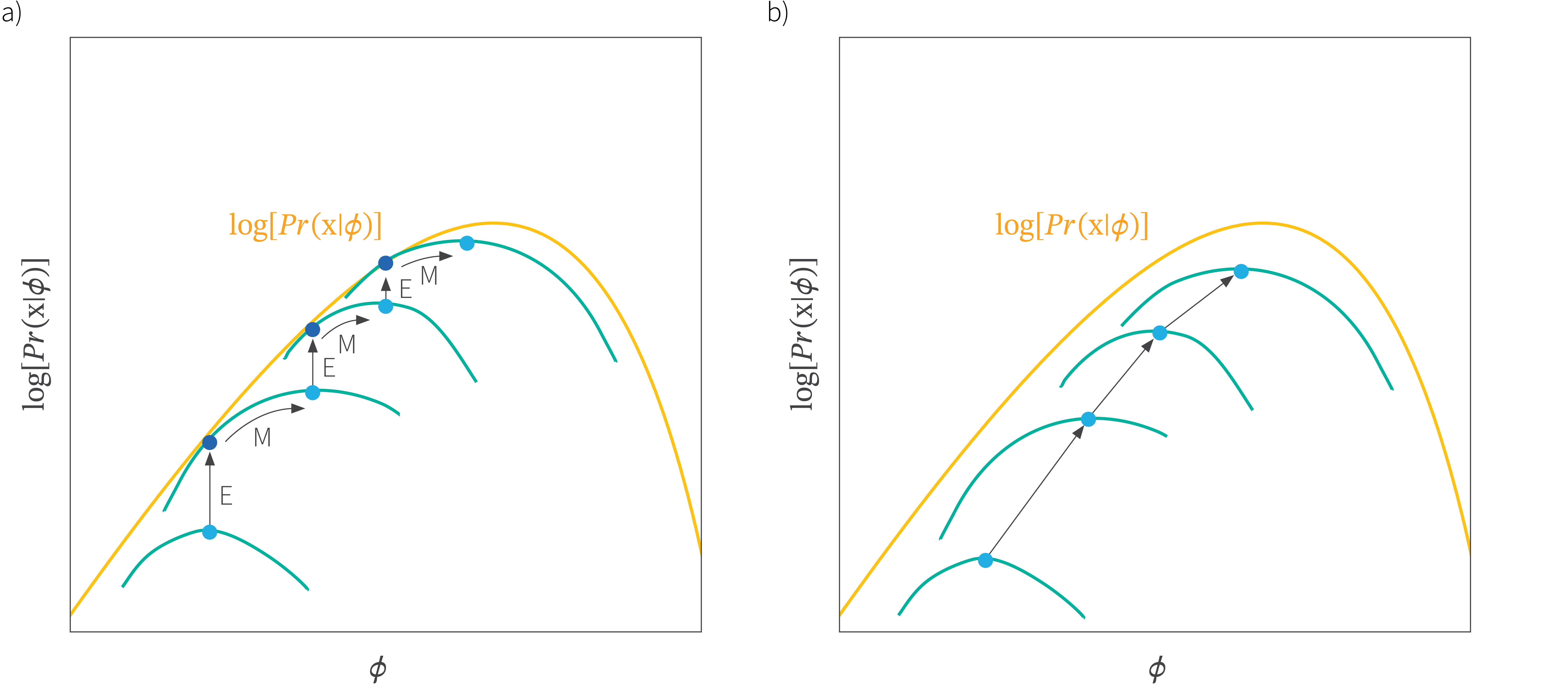
Figure 7. Expectation maximization vs. the VAE. a) Expectation maximization. In the EM algorithm, we alternately change the auxiliary parameters $\boldsymbol\theta$ (moving between green curves) and the main parameters $\boldsymbol\phi$ (moving along green curves) until we reach the overall maximum of the likelihood. These two types of change are known as the E-step and the M-step respectively. Because the E-Step uses the posterior distribution $Pr(h|\mathbf{x}, \boldsymbol\phi)$ for $q(h|\mathbf{x},\boldsymbol\theta)$, the bound is tight and so the green curve touches the yellow after each E-Step. b) In contrast the VAE changes both parameters at once and the bound is not in general tight so the green and yellow curves do not touch.
ELBO as reconstruction loss minus KL to prior
We’ve already seen two different ways to write the ELBO (equations 15 and 16). In fact, there are several more ways to re-express this function (see Hoffman & Johnson 2016). The one that is important for the VAE is:
\begin{eqnarray}\mbox{ELBO}[\boldsymbol\theta, \boldsymbol\phi] &=& \int q(\mathbf{h}|\boldsymbol\theta) \log\left[\frac{ Pr(\mathbf{x},\mathbf{h}|\boldsymbol\phi)}{q(\mathbf{h}|\boldsymbol\theta)} \right]d\mathbf{h}\nonumber \\&=& \int q(\mathbf{h}|\boldsymbol\theta) \log\left[\frac{ Pr(\mathbf{x}|\mathbf{h},\boldsymbol\phi)Pr(\mathbf{h})}{q(\mathbf{h}|\boldsymbol\theta)} \right]d\mathbf{h}\nonumber \\&=& \int q(\mathbf{h}|\boldsymbol\theta) \log\left[ Pr(\mathbf{x}|\mathbf{h},\boldsymbol\phi) \right]d\mathbf{h}+ \int q(\mathbf{h}|\boldsymbol\theta) \log\left[\frac{Pr(\mathbf{h})}{q(\mathbf{h}|\boldsymbol\theta)}\right]d\mathbf{h}\nonumber \\ &=& \int q(\mathbf{h}|\boldsymbol\theta) \log\left[ Pr(\mathbf{x}|\mathbf{h},\boldsymbol\phi) \right]d\mathbf{h}- \mbox{D}_{KL}[ q(\mathbf{h}|\boldsymbol\theta), Pr(\mathbf{h})] \tag{17}\end{eqnarray}
In this formulation, the first term measures the average agreement $Pr(\mathbf{x}|\mathbf{h},\boldsymbol\phi)$ of the hidden variable and the data (reconstruction loss) and the second one measures the degree to which the auxiliary distribution $q(\mathbf{h}, \boldsymbol\theta)$ matches the prior. This formulation is the one that will be used in the variational autoencoder.
The variational approximation
We have seen that the ELBO is tight when we choose the distribution $q(\mathbf{h}|\boldsymbol\theta)$ to be the posterior $Pr(\mathbf{h}|\mathbf{x},\boldsymbol\phi)$ but for the non-linear latent variable model, we cannot write an expression for this posterior.
The solution to the problem is to make a variational approximation: we just choose a simple parametric form for $q(\mathbf{h}|\boldsymbol\theta)$ and use this as an approximation to the true posterior. In this case we’ll choose a normal distribution with parameters $\boldsymbol\mu$ and $\boldsymbol\Sigma$. This distribution is not always going to be a great match to the posterior, but will be better for some values of $\boldsymbol\mu$ and $\boldsymbol\Sigma$ than others. When we optimize this model, we will be finding the normal distribution that is “closest” to the true posterior $Pr(\mathbf{h}|\mathbf{x})$ (figure 8). This corresponds to minimizing the KL divergence in equation 16.
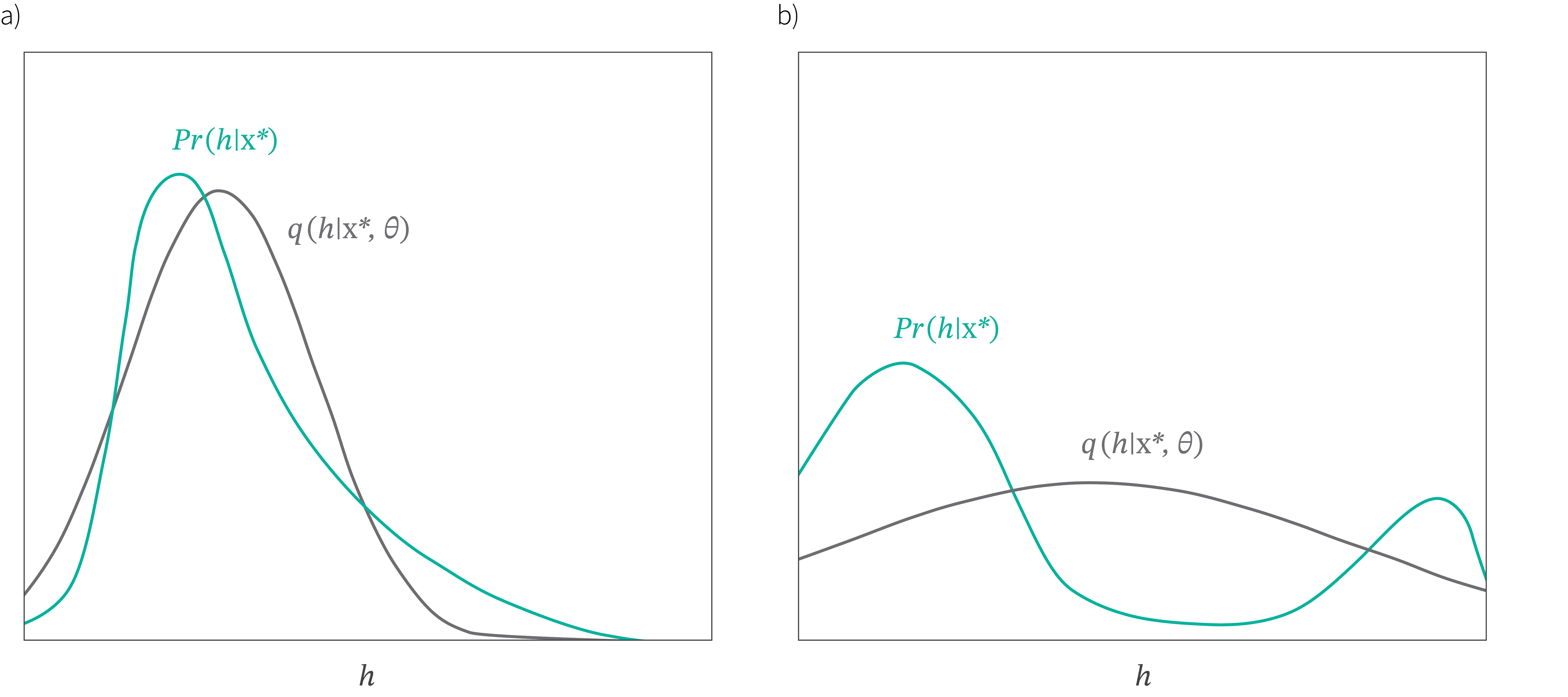
Figure 8. Variational approximation. The true posterior distribution $Pr(\mathbf{h}|\mathbf{x}^{*},\boldsymbol\phi)$ cannot be computed in closed form. The variational approximation chooses a particular family of distributions $q(\mathbf{h}|\mathbf{x},\boldsymbol\theta)$ (here Gaussian) and finds the closest member of this family to the true posterior. a) Sometimes this is a good approximation (i.e. the gray curve is close to the green one). b) However, if the posterior is multi-modal as in the example from figure 3, then the approximation will be poor.
Since the optimal choice for $q(\mathbf{h}|\boldsymbol\theta)$ was the posterior $Pr(\mathbf{h}|\mathbf{x})$ and this depended on the data example $\mathbf{x}$, it makes sense that our variational approximation should do the same and so we choose
\begin{equation}\label{eq:posterior_pred} q(\mathbf{h}|\boldsymbol\theta,\mathbf{x}) = \mbox{Norm}_{\mathbf{h}}[g_{\mu}[\mathbf{x}|\boldsymbol\theta], g_{\sigma}[\mathbf{x}|\boldsymbol\theta]], \tag{18}\end{equation}
where $g[\mathbf{x},\boldsymbol\theta]$ is a neural network with parameters $\boldsymbol\theta$ that predicts the mean and variance of the normal variational approximation.
The variational autoencoder
Finally, we are in a position to describe the variational autoencoder. We will build a network that computes the ELBO:
\begin{equation}\mbox{ELBO}[\boldsymbol\theta, \boldsymbol\phi] = \int q(\mathbf{h}|\mathbf{x},\boldsymbol\theta) \log\left[ Pr(\mathbf{x}|\mathbf{h},\boldsymbol\phi) \right]d\mathbf{h}- \mbox{D}_{KL}[ q(\mathbf{h}|\mathbf{x},\boldsymbol\theta), Pr(\mathbf{h})] \tag{19}\end{equation}
where the distribution $q(\mathbf{h}|\mathbf{x},\boldsymbol\theta)$ is the approximation from equation 18.
The first term in equation 19 still involves an integral that we cannot compute, but since it represents an expectation, we can approximate it with a set of samples:
\begin{equation}E[f[\mathbf{h}]] \approx \frac{1}{N}\sum_{n=1}^{N}f[\mathbf{h}^{*}_N]\tag{20}\end{equation}
where $\mathbf{h}^{*}_{n}$ is the $n^{th}$ sample. In the limit, we might only use a single sample $\mathbf{h}^{*}$ from $q(\mathbf{h}|\mathbf{x},\boldsymbol\theta)$ as a very approximate estimate of the expectation and here the ELBO will look like:
\begin{eqnarray}\mbox{ELBO}[\boldsymbol\theta, \boldsymbol\phi] &\approx& \log\left[ Pr(\mathbf{x}|\mathbf{h}^{*}|\boldsymbol\phi) \right]- \mbox{D}_{KL}[ q(\mathbf{h}|\mathbf{x},\boldsymbol\theta), Pr(\mathbf{h})] \tag{21}\end{eqnarray}
The second term is just the KL divergence between the variational Gaussian $q(\mathbf{h}|\mathbf{x},\boldsymbol\theta) = \mbox{Norm}_{\mathbf{h}}[\boldsymbol\mu,\boldsymbol\Sigma]$ and the prior $Pr(h) =\mbox{Norm}_{\mathbf{h}}[\mathbf{0},\mathbf{I}]$. The KL divergence between two Gaussians can be calculated in closed form and for this case is given by:
\begin{equation} \mbox{D}_{KL}[ q(\mathbf{h}|\mathbf{x},\boldsymbol\theta), Pr(\mathbf{h})] = \frac{1}{2}\left(\mbox{Tr}[\boldsymbol\Sigma] + \boldsymbol\mu^T\boldsymbol\mu – D – \log\left[\mbox{det}[\boldsymbol\Sigma]\right]\right). \tag{22}\end{equation}
were $D$ is the dimensionality of the hidden space.
So, to compute the ELBO for a point $\mathbf{x}$ we first estimate the mean $\boldsymbol\mu$ and variance $\boldsymbol\Sigma$ of the posterior distribution $q(\mathbf{h}|\boldsymbol\theta,\mathbf{x})$ for this data point $\mathbf{x}$ using the network $\mbox{g}[\mathbf{x},\boldsymbol\theta]$. Then we draw a sample $\mathbf{h}^{*}$ from this distribution. Finally, we compute the ELBO using equation 21.
The architecture to compute this is shown in figure 9. Now it’s clear why it is called a variational autoencoder. It is an autoencoder because it starts with a data point $\mathbf{x}$, computes a lower dimensional latent vector $\mathbf{h}$ from this and then uses this to recreate the original vector $\mathbf{x}$ as closely as possible. It is variational because it computes a Gaussian approximation to the posterior distribution along the way.
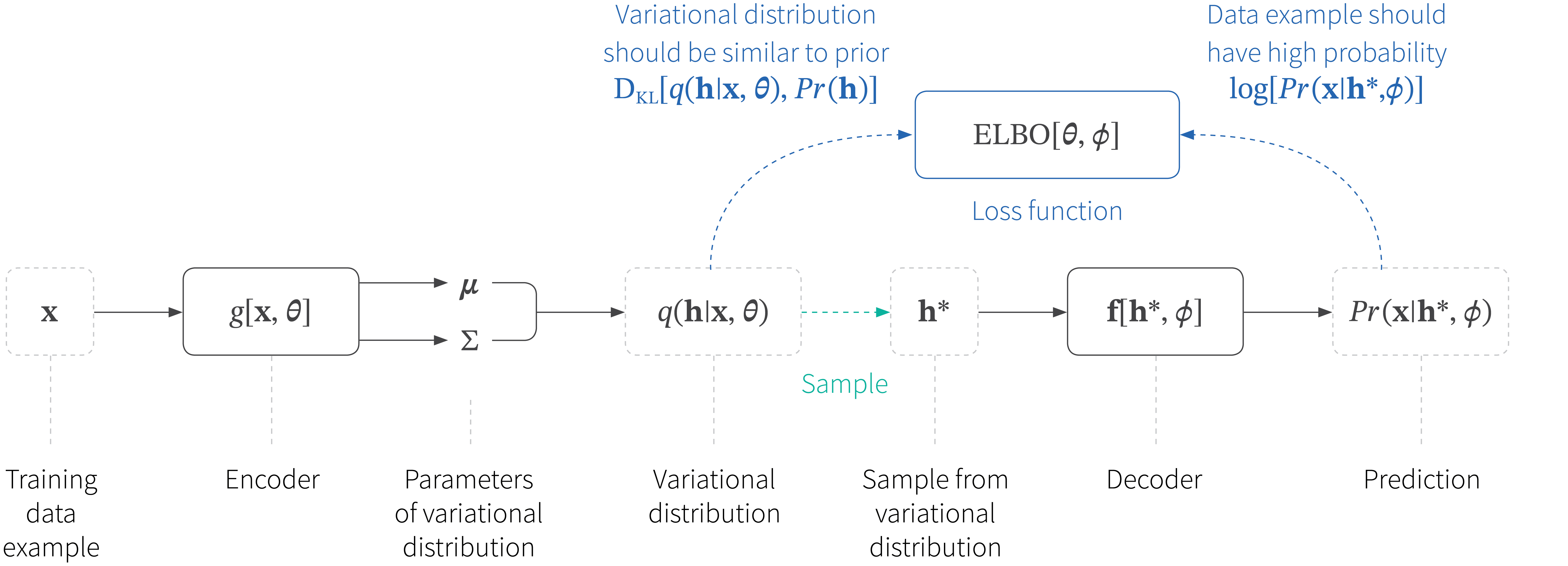
Figure 9. Variational autoencoder. The encoder takes the training data and predicts the parameters (mean and covariance) of the variational distribution. We sample from this distribution and then use the decoder to make a prediction for the data based on this sample. The cost function is the ELBO that depends on how good this prediction is and how similar the variational distribution is to the prior.
The VAE computes the ELBO bound as a function of the parameters $\boldsymbol\phi$ and $\boldsymbol\theta$. When we maximize this bound as a function of both of these parameters, we gradually move the parameters $\boldsymbol\phi$ to values that have give the data a higher likelihood under the non-linear latent variable model (figure 7b).
In this section, we’ve described how to compute the ELBO for a single point, but actually we want to maximize its sum over all of the data examples. As in most deep learning methods, we accomplish this with stochastic gradient descent, by running mini-batches of points through our network.
The reparameterization trick
You might think that we are done; we set up this architecture, then we allow PyTorch / Tensorflow to perform automatic differentiation via the backpropagation algorithm and hence optimize the cost function. However, there’s a problem. The network involves a sampling step and there is no way to differentiate through this. Consequently, it’s impossible to make updates to the parameters $\boldsymbol\theta$ that occur earlier in the network than this.
Fortunately, there is a simple solution; we can move the stochastic part into a branch of the network which draws a sample from $\mbox{Norm}_{\epsilon}[\mathbf{0},\mathbf{I}]$ and then use the relation
\begin{equation} \mathbf{h}^{*} = \boldsymbol\mu + \boldsymbol\Sigma^{1/2}\epsilon, \tag{23}\end{equation}
to draw from the intended Gaussian. Now we can compute the derivatives as usual because there is no need for the backpropagation algorithm to pass down the stochastic branch. This is known as the reparameterization trick and is illustrated in figure 10.
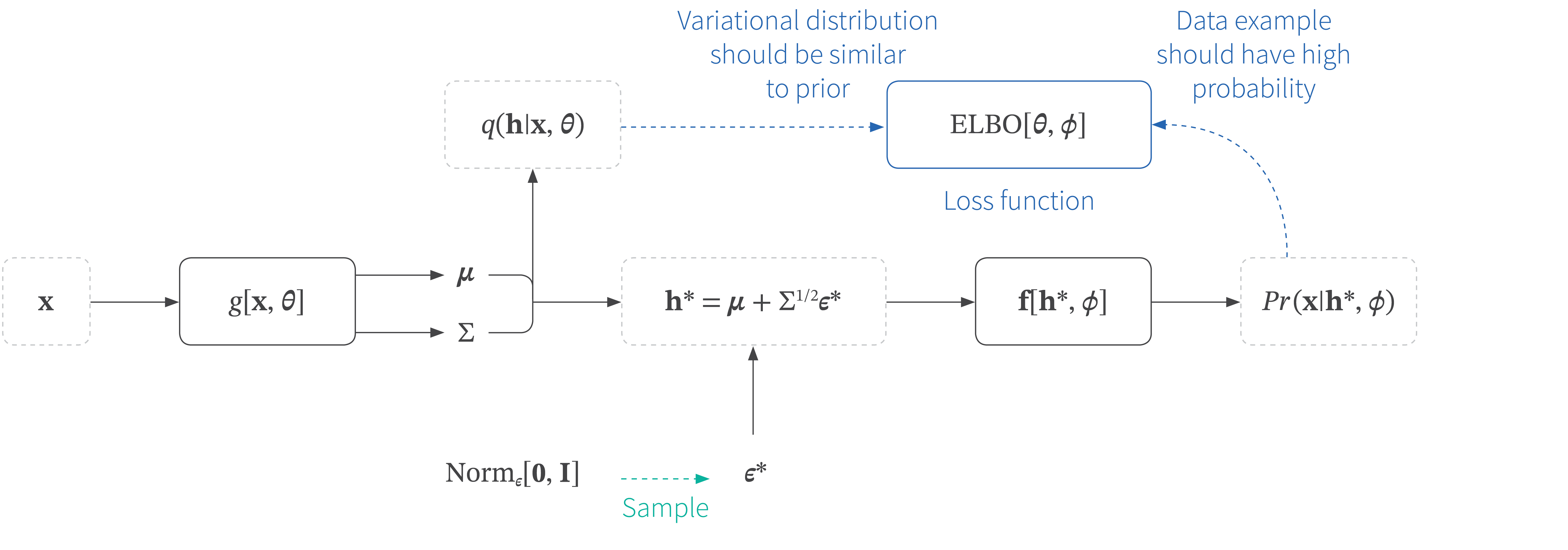
Figure 10. Reparameterization trick. With the original architecture (figure 9), we cannot backpropagate through the sampling step. The reparameterization trick removes the sampling step from the main pipeline so that we can backpropagate. Instead we sample from a standard normal and combine this with the predicted mean and covariance to get a sample from the variational distribution.
Extensions to VAEs
Variational autoencoders were first introduced by Kingma &Welling (2013). Since then, they have been extended in several ways. First, they have been adapted to other data types including discrete data (van den Oord et al. 2017, Razavi et al. 2019), word sequences (Bowman et al. 2015), and temporal data (Gregor & Besse 2018). Second, researchers have experimented with different forms for the variational distribution, most notably using normalizing flows which can approximate the true posterior much more closely than a Gaussian (Rezende & Mohamed 2015). Third, there is a strand of work investigating more complex likelihood models $Pr(\mathbf{x}|\mathbf{h})$. For example, Gulrajani et al. (2016) used an auto-regressive relation between output variables and Dorta et al. (2018) modeled the covariance as well as the mean.
Finally, there is a large body of work that attempts to improve the properties of the latent space. Here, one popular goal is to learn a disentangled representation in which each dimension of the latent space represents an independent real world factor. For example, when modeling face images, we might hope to uncover head pose or hair color as independent factors. These methods generally add regularization terms to either the posterior $q(\mathbf{h}|\mathbf{x})$ or the aggregated posterior $q(\mathbf{h}) = \frac{1}{J}\sum_{i=1}^{I}q(\mathbf{h}|\mathbf{x}_{i})$ so that the new loss function is
\begin{equation} L_{new} = \mbox{ELBO}[\boldsymbol\theta, \boldsymbol\phi] – \lambda_{1} \mathbb{E}_{Pr(\mathbf{x})}\left[\mbox{R}_{1}\left[q(\mathbf{h}|\mathbf{x}) \right]\right] – \lambda_{2} \mbox{R}_{2}[q(\mathbf{h})], \tag{24}\end{equation}
where $\lambda_{1}$ and $\lambda_{2}$ are weights and $\mbox{R}_{1}[\bullet]$ and $\mbox{R}_{2}[\bullet]$ are functions of the posterior and aggregated posterior respectively. This class of methods includes the BetaVAE (Higgins et al. 2017), InfoVAE (Zhao et al. 2017) and many others (e.g., Kim & Mnih 2018, Kumar et al. 2017, Chen et al. 2018).
Problems with VAEs
VAEs have several drawbacks. First, we cannot compute the likelihood of a new point $\mathbf{x}$ under the probability distribution efficiently, because this involves integrating over the hidden variable $\mathbf{h}$. We can approximate this integral using a Markov chain Monte Carlo method, but this is very inefficient. Second, samples from VAEs are generally not perfect (figure 11). The naive spherical Gaussian noise model which is independent for each variable generally produces noisy samples (or overly smooth ones if we do not add in the noise).
In practice, training VAEs (particularly sequence VAEs) can be brittle. It’s possible that that the system converges to a local minimum in which the latent variable is completely ignored and the encoder always predicts the prior. This phenomenon is known as posterior collapse (Bowman et al. 2015). One way to avoid this problem is to only gradually introduce the second term in the cost function (equation 19) using an annealing schedule.
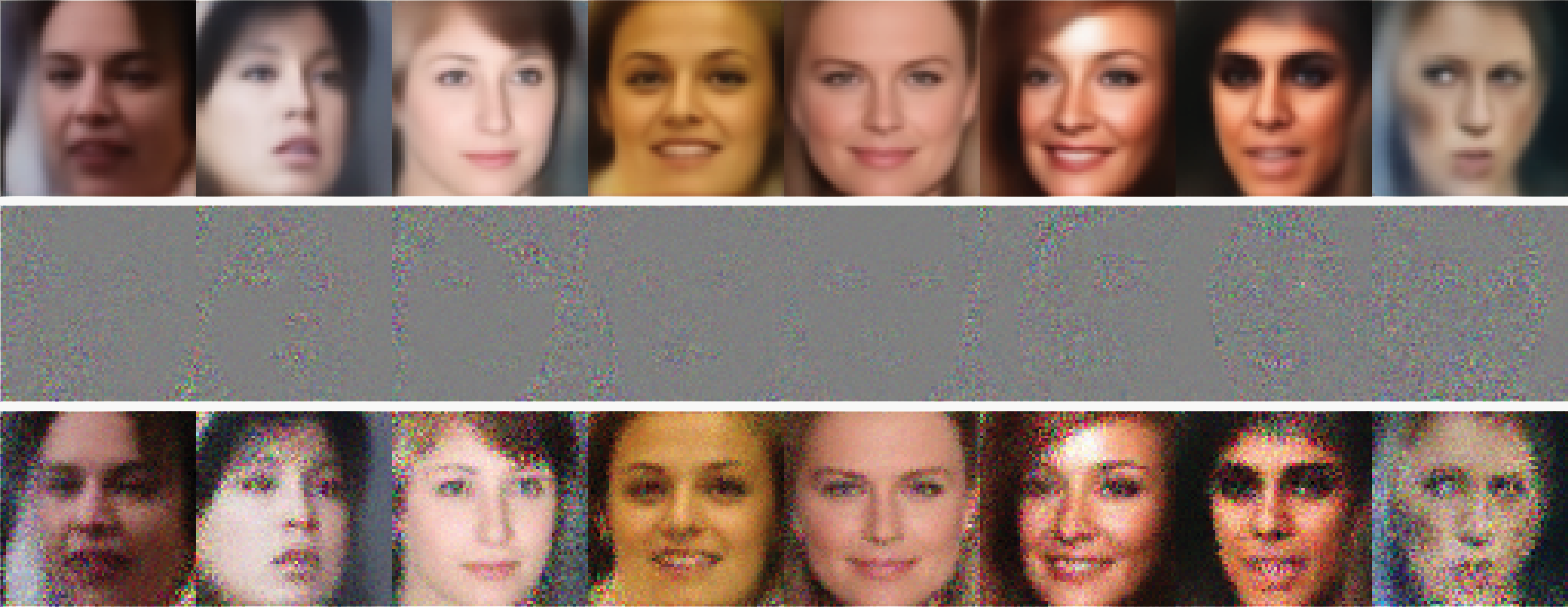
Figure 11. Sampling from a VAE trained on CELEBA faces dataset. In each column we draw a random value of the latent variable $\mathbf{h}$ and then used this to predict the mean $\mbox{f}[\mathbf{h}^{*},\boldsymbol\phi]$ of the pixel data. The first row shows examples of these means. The second row shows an instantiation of the per-pixel spherical Gaussian noise and the third row shows the sum of the first two rows and is the final sample. The images look over-smooth before we add the noise and over-noisy once we add it. This is a typical drawback of using VAEs to sample images. Reproduced with permission from Dorta 2019 — Learning models for intelligent photo-editing.
Summary
The VAE is an architecture to learn a probability model over $Pr(\mathbf{x})$. This model can generate samples, and interpolate between them (by manipulating the latent variable $\mathbf{h}$) but it is not easy to compute the likelihood for a new example. There are two main alternatives to the VAE. The first is generative adversarial networks. These are good for sampling but their samples have quite different properties from those produced by the VAE. Similarly to the VAE they cannot evaluate the likelihood of new data points. The second alternative is normalizing flows for which the both sampling and likelihood evaluation are tractable.
Work with Us!
Impressed by the work of the team? RBC Borealis is looking to hire for various roles across different teams. Visit our career page now and discover opportunities to join similar impactful projects!
Careers at RBC Borealis