
Optimization is at the heart of machine learning. When we fit a model, we rely on finding the minimum of the associated cost function. Fortunately, many optimization problems are relatively easy. For example, the cost function for a logistic regression model is convex with a single minimum and closed-form derivatives and so any sensible gradient-based method will find the minimum.
However, other optimization problems are much more challenging. Consider hyperparameter search in a neural network. Before we a train the network, we must choose the architecture, optimization algorithm, and cost function. These choices are encoded numerically as a vector of hyperparameters. To get the best performance, we must find the hyperparameters for which the resulting trained network is best. This hyperparameter optimization problem has many challenging characteristics:
Evaluation cost: Evaluating the function that we wish to maximize (i.e., the network performance) in hyperparameter search is very expensive; we have to train the neural network model and then run it on the validation set to measure the network performance for a given set of hyperparameters.
Multiple local optima: The function is not convex and there may be many combinations of hyperparameters that are locally optimal.
No derivatives: We do not have access to the gradient of the function with respect to the hyperparameters; there is no easy and inexpensive way to propagate gradients back through the model training / validation process.
Variable types: There are a mixture of discrete variables (e.g., the number of layers, number of units per layer and type of non-linearity) and continuous variables (e.g., the learning rate and regularization weights).
Conditional variables: The existence of some variables depends on the settings of others. For example, the number of units in layer $3$ is only relevant if we already chose $\geq 3$ layers.
Noise: The function may return different values for the same input hyperparameter set. The neural network training process relies on stochastic gradient descent and so we typically don’t get exactly the same result every time.
Bayesian optimization is a framework that can deal with optimization problems that have all of these challenges. The core idea is to build a model of the entire function that we are optimizing. This model includes both our current estimate of that function and the uncertainty around that estimate. By considering this model, we can choose where next to sample the function. Then we update the model based on the observed sample. This process continues until we are sufficiently certain of where the best point on the function is.
Problem setup
Let’s now put aside the specific example of hyperparameter search and consider Bayesian optimization in its more general form. Bayesian optimization addresses problems where the aim is to find the parameters $\hat{\mathbf{x}}$ that maximize a function $\mbox{f}[\mathbf{x}]$ over some domain $\mathcal{X}$ consisting of finite lower and upper bounds on every variable:
\begin{equation}\hat{\mathbf{x}} = \mathop{\rm argmax}_{\mathbf{x} \in \mathcal{X}} \left[ \mbox{f}[\mathbf{x}]\right]. \tag{1}\label{eq:global-opt}\end{equation}
At iteration $t$, the algorithm can learn about the function by choosing parameters $\mathbf{x}_t$ and receiving the corresponding function value $f[\mathbf{x}_t]$. The goal of Bayesian optimization is to find the maximum point on the function using the minimum number of function evaluations. More formally, we want to minimize the number of iterations $t$ before we can guarantee that we find parameters $\hat{\mathbf{x}}$ such $f[\hat{\mathbf{x}}]$ is less than $\epsilon$ from the true maximum $\hat{f}$.
Simple strategies
We’ll assume for now that all parameters are continuous, that their existences are not conditional on one another, and that the cost function is deterministic so that it always returns the same value for the same input. We’ll return these complications later in this document. To help understand the basic optimization problem let’s consider some simple strategies:
Grid Search: One obvious approach is to quantize each dimension of $\mathbf{x}$ to form an input grid and then evaluate each point in the grid (figure 1). This is simple and easily parallelizable, but suffers from the curse of dimensionality; the size of the grid grows exponentially in the number of dimensions.

Figure 1. Grid search vs. random search. a) Grid search. In grid search we sample each parameter regularly. However, in this case one of the parameters has little effect on the cost function. Because we sampled in a grid, we have only tried three values of the important variable in nine function evaluations. b) Random search. Here, we sample the function randomly and hence try nine different values of the important variable in nine function evaluations. Adapted from Bergstra and Bengio (2012).
Random Search: Another strategy is to specify probability distributions for each dimension of $\mathbf{x}$ and then randomly sample from these distributions (Bergstra and Bengio, 2012). This addresses a subtle inefficiency of grid search that occurs when one of the parameters has very little effect on the function output (see figure 1 for details). Random search is also simple and parallelizable. However, if we are unlucky, we can may either (i) make many similar observations that provide redundant information, or (ii) never sample close to the global maximum.
Sequential search strategies: One obvious deficiency of both grid search and random search is that they do not take into account previous measurements. If the measurements are made sequentially then we could use the previous results to decide where it might be strategically best to sample next (figure 2). One idea is that we could explore areas where there are few samples so that we are less likely to miss the global maximum entirely. Another approach could exploit what we have learned so far by sampling more in relatively promising areas. An optimal strategy would recognize that there is a trade-off between exploration and exploitation and combine both ideas.
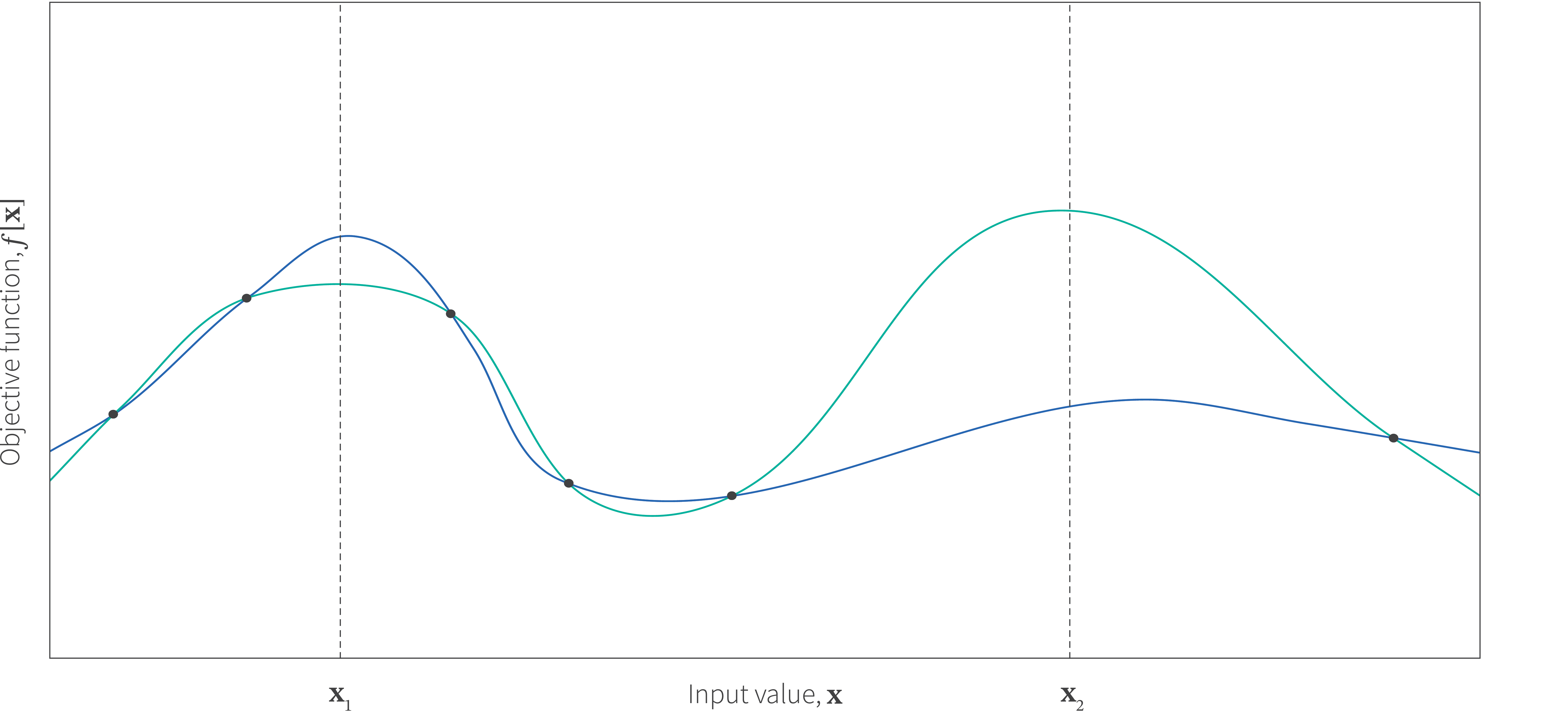
Figure 2. Exploration vs. exploitation. Consider a one-dimensional objective function $f[\mathbf{x}]$, from which we have already sampled five points (black circles). Where should we sample next? We could sample at position $\mathbf{x}_{1}$ which is close to the best points we have seen so far and we might potentially find a better point still. Alternatively, we could sample at position at $\mathbf{x}_{2}$, exploring a part of the function that we have not yet measured and perhaps it will turn out that the function will return an even better value here. Of course, the best strategy depends on the underlying function (which we don’t know). If the function is like the blue curve then the first strategy is better. However, if it is more like the green curve then the second strategy is superior.
Bayesian Optimization
Bayesian optimization is a sequential search framework that incorporates both exploration and exploitation and can be considerably more efficient than either grid search or random search. It can easily be motivated from figure 2; the goal is to build a probabilistic model of the underlying function that will know both (i) that $\mathbf{x}_{1}$ is a good place to sample because the function will probably return a high value here and (ii) that $\mathbf{x}_{2}$ is a good place to sample because the uncertainty here is very large.
A Bayesian optimization algorithm has two main components:
- A probabilistic model of the function: Bayesian optimization starts with an initial probability distribution (the prior) over the function $f[\bullet]$ to be optimized. Usually this just reflects the fact that we are extremely uncertain about what the function is. With each observation of the function $(\mathbf{x}_t, f[\mathbf{x}_t])$, we learn more and the distribution over possible functions (now called the posterior) becomes narrower.
- An acquisition function: This is computed from the posterior distribution over the function and is defined on the same domain. The acquisition indicates the desirability of sampling each point next and depending on how it is defined it can favor exploration or exploitation.
In the next two sections, we consider each of these components in turn.
A model of the function: Gaussian processes
There are several ways to model the function and its uncertainty, but the most popular approach is to use Gaussian processes (GPs). We will present other models (Bernoulli-Beta bandits, random forests, and Tree-Parzen estimators) later in this document.
A Gaussian Process is a collection of random variables, where any finite number of these are jointly normally distributed. It is defined by (i) a mean function $\mbox{m}[\mathbf{x}]$ and (ii) a covariance function $k[\mathbf{x},\mathbf{x}’]$ that returns the similarity between two points. When we model our function as $\mbox{f}[\mathbf{x}]\sim \mbox{GP}[\mbox{m}[\mathbf{x}],k[\mathbf{x},\mathbf{x}^\prime]]$ we are saying that:
\begin{eqnarray}\mathbb{E}[\mbox{f}[\mathbf{x}]] &=& \mbox{m}[\mathbf{x}] \tag{2}\end{eqnarray}
\begin{eqnarray}\mathbb{E}[(\mbox{f}[\mathbf{x}]-\mbox{m}[\mathbf{x}])(f[\mathbf{x}’]-\mbox{m}[\mathbf{x}’])] &=& k[\mathbf{x}, \mathbf{x}’]. \tag{3}\end{eqnarray}
The first equation states that the expected value of the function is given by some function $\mbox{m}[\mathbf{x}]$ of $\mathbf{x}$ and the second equation tells us how to compute the covariance of any two points $\mathbf{x}$ and $\mathbf{x}’$. As a concrete example, let’s choose:
\begin{eqnarray}\mbox{m}[\mathbf{x}] &=& 0 \tag{4}\end{eqnarray}
\begin{eqnarray}k[\mathbf{x}, \mathbf{x}’] &=&\mbox{exp}\left[-\frac{1}{2}\left(\mathbf{x}-\mathbf{x}’\right)^{T}\left(\mathbf{x}-\mathbf{x}’\right)\right], \tag{5}\end{eqnarray}
so here the expected function values are all zero and the covariance decreases as a function of distance between two points. In other words, points very close to one another of the function will tend to have similar values and those further away will be less similar.
Given observations $\mathbf{f} = [f[\mathbf{x}_{1}], f[\mathbf{x}_{2}],\ldots, f[\mathbf{x}_{t}]]$ at $t$ points, we would like to make a prediction about the function value at a new point $\mathbf{x}^{*}$. This new function value $f^{*} = f[\mathbf{x}^{*}]$ is jointly normally distributed with the observations $\mathbf{f}$ so that:
\begin{equation}Pr\left(\begin{bmatrix}\label{eq:GP_Joint}\mathbf{f}\\f^{*}\end{bmatrix}\right) = \mbox{Norm}\left[\mathbf{0}, \begin{bmatrix}\mathbf{K}[\mathbf{X},\mathbf{X}] & \mathbf{K}[\mathbf{X},\mathbf{x}^{*}]\\ \mathbf{K}[\mathbf{x}^{*},\mathbf{X}]& \mathbf{K}[\mathbf{x}^{*},\mathbf{x}^{*}]\end{bmatrix}\right], \tag{6}\end{equation}
where $\mathbf{K}[\mathbf{X},\mathbf{X}]$ is a $t\times t$ matrix where element $(i,j)$ is given by $k[\mathbf{x}_{i},\mathbf{x}_{j}]$, $\mathbf{K}[\mathbf{X},\mathbf{x}^{*}]$ is a $t\times 1$ vector where element $i$ is given by $k[\mathbf{x}_{i},\mathbf{x}^{*}]$ and so on.
Since the function values in equation 6 are jointly normal, the conditional distribution $Pr(f^{*}|\mathbf{f})$ must also be normal, and we can use the standard formula for the mean and variance of this conditional distribution:
\begin{equation}\label{eq:gp_posterior}Pr(f^*|\mathbf{f}) = \mbox{Norm}[\mu[\mathbf{x}^{*}],\sigma^{2}[\mathbf{x}^{*}]], \tag{7}\end{equation}
where
\begin{eqnarray}\label{eq:GP_Conditional}\mu[\mathbf{x}^{*}]&=& \mathbf{K}[\mathbf{x}^{*},\mathbf{X}]\mathbf{K}[\mathbf{X},\mathbf{X}]^{-1}\mathbf{f}\nonumber \\\sigma^{2}[\mathbf{x}^{*}]&=&\mathbf{K}[\mathbf{x}^{*},\mathbf{x}^{*}]\!-\!\mathbf{K}[\mathbf{x}^{*}, \mathbf{X}]\mathbf{K}[\mathbf{X},\mathbf{X}]^{-1}\mathbf{K}[\mathbf{X},\mathbf{x}^{*}]. \tag{8}\end{eqnarray}
Using this formula, we can estimate the distribution of the function at any new point $\mathbf{x}^{*}$. The best estimate of the function value is given by the mean $\mu[\mathbf{x}]$, and the uncertainty is given by the variance $\sigma^{2}[\mathbf{x}]$. Figure 3 shows an example of measuring several points on a function sequentially and showing how the predicted mean and variance changes for other points.

Figure 3. Gaussian process model. a) Consider a case where we have sampled four points of a function at positions $x_{1}$, $x_{2}$, $x_{3}$ and $x_{4}$. The Gaussian process model describes a probability distribution over possible functions that pass through these four points. This can be visualized as a mean function $\mu[\mathbf{x}^{*}]$ (blue curve) and an uncertainty around that mean at each point $\sigma^{2}[x]$ (gray region). b-d) As we sequentially add points, the mean of the function changes to pass smoothly through the new points and the uncertainty decreases in response to the extra information that each point brings.
Acquisition functions
Now that we have a model of the function and its uncertainty, we will use this to choose which point to sample next. The acquisition function takes the mean and variance at each point $\mathbf{x}$ on the function and computes a value that indicates how desirable it is to sample next at this position. A good acquisition function should trade off exploration and exploitation.
In the following sections we’ll describe four popular acquisition functions: the upper confidence bound (Srinivas et al., 2010), expected improvement (Močkus, 1975), probability of improvement (Kushner, 1964), and Thompson sampling (Thompson, 1933). Note that there are several other approaches which are not discussed here including those based on entropy search (Villemonteix et al., 2009, Hennig and Schuler, 2012) and the knowledge gradient (Wu et al., 2017).
Upper confidence bound: This acquisition function (figure 4a) is defined as:
\begin{align}\mbox{UCB}[\mathbf{x}^{*}] = \mu[\mathbf{x}^{*}] + \beta^{1/2} \sigma[\mathbf{x}^{*}]. \label{eq:UCB-def} \tag{9}
\end{align}
This favors either (i) regions where $\mu[\mathbf{x}^{*}]$ is large (for exploitation) or (ii) regions where $\sigma[\mathbf{x}^{*}]$ is large (for exploration). The positive parameter $\beta$ trades off these two tendencies.

Figure 2. Exploration vs. exploitation. Consider a one-dimensional objective function $f[\mathbf{x}]$, from which we have already sampled five points (black circles). Where should we sample next? We could sample at position $\mathbf{x}_{1}$ which is close to the best points we have seen so far and we might potentially find a better point still. Alternatively, we could sample at position at $\mathbf{x}_{2}$, exploring a part of the function that we have not yet measured and perhaps it will turn out that the function will return an even better value here. Of course, the best strategy depends on the underlying function (which we don’t know). If the function is like the blue curve then the first strategy is better. However, if it is more like the green curve then the second strategy is superior.
Probability of improvement: This acquisition function computes the likelihood that the function at $\mathbf{x}^{*}$ will return a result higher than the current maximum $\mbox{f}[\hat{\mathbf{x}}]$. For each point $\mathbf{x}^{*}$, we integrate the part of the associated normal distribution that is above the current maximum (figure 4b) so that:
\begin{equation} \mbox{PI}[\mathbf{x}^{*}] = \int_{\mbox{f}[\hat{\mathbf{x}}]}^{\infty} \mbox{Norm}_{\mbox{f}[\mathbf{x}^{*}]}[\mu[\mathbf{x}^{*}],\sigma[\mathbf{x}^{*}]] d\mbox{f}[\mathbf{x}^{*}] \tag{10}\end{equation}
Expected improvement: The main disadvantage of the probability of improvement function is that it does not take into account how much the improvement will be; we do not want to favor small improvements (even if they are very likely) over larger ones. Expected improvement (figure 4c) takes this into account. It computes the expectation of the improvement $f[\mathbf{x}^{*}]- f[\hat{\mathbf{x}}]$ over the part of the normal distribution that is above the current maximum to give:
\begin{equation} \mbox{EI}[\mathbf{x}^{*}] = \int_{\mbox{f}[\hat{\mathbf{x}}]}^{\infty} (f[\mathbf{x}^{*}]- f[\hat{\mathbf{x}}])\mbox{Norm}_{\mbox{f}[\mathbf{x}^{*}]}[\mu[\mathbf{x}^{*}],\sigma[\mathbf{x}^{*}]] d\mbox{f}[\mathbf{x}^{*}]. \tag{11}\end{equation}
There also exist methods to allow us to trade-off exploitation and exploration for probability of improvement and expected improvement (see Brochu et al., 2010).
Thompson sampling: When we introduced Gaussian processes, we only talked about how to compute the probability distribution for a single new point $\mathbf{x}^{*}$. However, it’s also possible to draw a sample from the joint distribution of many new points that could collectively represent the entire function. Thompson sampling (figure 4d) exploits this by drawing such a sample from the posterior distribution over possible functions and then chooses the next point $\mathbf{x}$ according to the position of the maximum of this sampled function. To draw the sample, we append an equally spaced set of points to the observed ones as in equation 6, use the conditional formula to find a Gaussian distribution over these points as in equation 8, and then draw a sample from this Gaussian.
Worked example
Figure 5 shows a complete worked example of Bayesian optimization in one dimension using the upper confidence bound. As we sample more points, the function becomes steadily more certain. The method explores the function but also focuses on promising areas, exploiting what it has already learned.
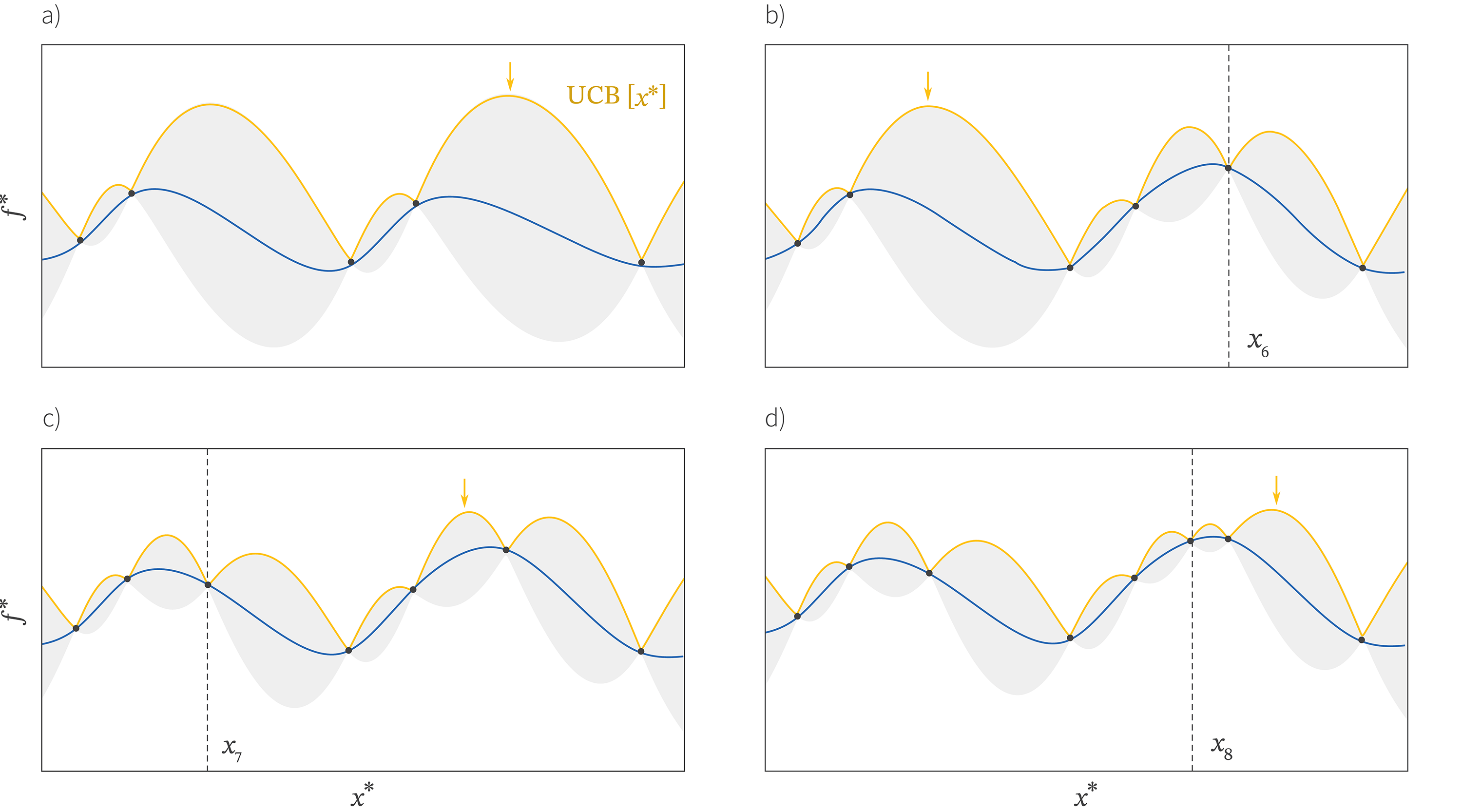
Figure 5. Bayesian optimization worked example using the upper confidence bound. a) Gaussian process model of five points. The upper confidence bound (yellow line) with parameter $\beta=4$ is given by the upper limit of the shaded area. We find the maximum point (yellow arrow) and sample the function here. b) The resulting pair $(x_{6},f[x_{6}])$ causes the model to be refined and the uncertainty to decrease close to the new point. The new maximum of the upper confidence bound is hence in a quite different place. c)-d) As this process continues, we add more points and the uncertainty around the function (grey area) decrease. Notice that the algorithm explores new regions (panels b and c) and also exploits promising regions (panel d).
Bayesian optimization with GPs in practice
In the previous section, we summarized the main ideas of Bayesian optimization with Gaussian processes. In this section, we’ll dig a bit deeper into some of the practical aspects. We consider how to deal with noisy observations, how to choose a kernel, how to learn the parameters of that kernel, how to exploit parallel sampling of the function, and finally we’ll discuss some limitations of the approach.
Incorporating noisy measurements
Until this point, we have assumed that the function that we are estimating is noise-free and always returns the same value $\mbox{f}[\mathbf{x}]$ for a given input $\mathbf{x}$. To incorporate a stochastic output with variance $\sigma_{n}^{2}$, we add an extra noise term to the expression for the Gaussian process covariance:
\begin{eqnarray}\mathbb{E}[(y[\mathbf{x}]-\mbox{m}[\mathbf{x}])(y[\mathbf{x}]-\mbox{m}[\mathbf{x}’])] &=& k[\mathbf{x}, \mathbf{x}’] + \sigma^{2}_{n}. \tag{12}\end{eqnarray}
We no longer observe the function values $\mbox{f}[\mathbf{x}]$ directly, but observe noisy corruptions $y[\mathbf{x}] = \mbox{f}[\mathbf{x}]+\epsilon$ of them. The joint distribution of previously observed noisy function values $\mathbf{y}$ and a new unobserved point $f^{*}$ becomes:
\begin{equation}Pr\left(\begin{bmatrix}\mathbf{y}\\f^{*}\end{bmatrix}\right) = \mbox{Norm}\left[\mathbf{0}, \begin{bmatrix}\mathbf{K}[\mathbf{X},\mathbf{X}]+\sigma^{2}_{n}\mathbf{I} & \mathbf{K}[\mathbf{X},\mathbf{x}^{*}]\\ \mathbf{K}[\mathbf{x}^{*},\mathbf{X}]& \mathbf{K}[\mathbf{x}^{*},\mathbf{x}^{*}]\end{bmatrix}\right], \tag{13}\end{equation}
and the conditional probability of a new point becomes:
\begin{eqnarray}\label{eq:noisy_gp_posterior}Pr(f^{*}|\mathbf{y}) &=& \mbox{Norm}[\mu[\mathbf{x}^{*}],\sigma^{2}[\mathbf{x}^{*}]], \tag{14}\end{eqnarray}
where
\begin{eqnarray}\mu[\mathbf{x}^{*}]&=& \mathbf{K}[\mathbf{x}^{*},\mathbf{X}](\mathbf{K}[\mathbf{X},\mathbf{X}]+\sigma^{2}_{n}\mathbf{I})^{-1}\mathbf{f}\nonumber \\\sigma^{2}[\mathbf{x}^{*}] &=& \mathbf{K}[\mathbf{x}^{*},\mathbf{x}^{*}]\!-\!\mathbf{K}[\mathbf{x}^{*}, \mathbf{X}](\mathbf{K}[\mathbf{X},\mathbf{X}]+\sigma^{2}_{n}\mathbf{I})^{-1}\mathbf{K}[\mathbf{X},\mathbf{x}^{*}]. \tag{15}\end{eqnarray}
Incorporating noise means that there is uncertainty about the function even where we have already sampled points (figure 6), and so sampling twice at the same position or at very similar positions could be sensible.

Figure 6. Incorporating noisy measurements. a) In our original presentation we assumed that the function always returns the same answer for the same input. This means that the mean of our GP model must pass exactly through every point and the function uncertainty at every sample point is zero. b) If we assume that there is measurement noise, then this constraint is relaxed. Notice that the uncertainty is smaller closer to the samples, but is not zero. In the context of Bayesian optimization this means that it could be sensible to sample the same position more than once.
Kernel choice
When we build the model of the function and its uncertainty, we are assuming that the function is smooth. If this was not the case, then we could say nothing at all about the function between the sampled points. The details of this smoothness assumption are embodied in the choice of kernel covariance function.
We can visualize the covariance function by drawing samples from the Gaussian process prior. In one dimension, we do this by defining an evenly spaced set of points $\mathbf{X}=\begin{bmatrix}\mathbf{x}_{1},& \mathbf{x}_{2},&\cdots,& \mathbf{x}_{I}\end{bmatrix}$, drawing a sample from $\mbox{Norm}[\mathbf{0}, \mathbf{K}[\mathbf{X},\mathbf{X}]]$ and then plotting the results. In this section, we’ll consider several different choices of covariance function, and use this method to visualize each.
Squared Exponential Kernel: In our example above, we used the squared exponential kernel, but more properly we should have included the amplitude $\alpha$ which controls the overall amount of variability and the length scale $\lambda$ which controls the amount of smoothness:
\begin{equation}\label{eq:bo_squared_exp}\mbox{k}[\mathbf{x},\mathbf{x}’] = \alpha^{2}\cdot \mbox{exp}\left[-\frac{d^{2}}{2\lambda}\right],\nonumber \end{equation}
where $d$ is the Euclidean distance between the points:
\begin{equation}d = \sqrt {\left(\mathbf{x}-\mathbf{x}’\right)^{T}\left(\mathbf{x}-\mathbf{x}’\right)}. \tag{16}\end{equation}
When the amplitude $\alpha^{2}$ is small, the function does not vary too much in the vertical direction. When it is larger, there is more variation. When the length scale $\lambda$ is small, the function is assumed to be less smooth and we quickly become uncertain about the state of the function as we move away from known positions. When it is large, the function is assumed to be more smooth and we are increasingly confident about what happens away from these observations (figure 7). Samples from the squared exponential kernel are visualized in figure 8a-c.

Figure 7. Effect of kernel length scale. a) When the length scale $\lambda$ is small, the function changes quickly and fits through all of the points exactly. The uncertainty increases very quickly as we depart from an observed point. b-c) As the length scale increases, the mean of the function becomes smoother, but does not fit through all the points exactly. The uncertainty away from observed points increases more slowly.
Matérn kernel: The squared exponential function assumes that the function is infinitely differentiable. The Matérn kernel (figure 8d-l) relaxes this constraint by assuming a certain degree of smoothness $\nu$. The Matérn kernel with $\nu=0.5$ is once differentiable and is defined as
\begin{equation}\mbox{k}[\mathbf{x},\mathbf{x}’] = \alpha^{2}\cdot \exp\left[-\frac{d}{\lambda^{2}}\right], \tag{17}\end{equation}
where once again, $d$ is the Euclidean distance between $\mathbf{x}$ and $\mathbf{x}’$, $\alpha$ is the amplitude, and $\lambda$ is the length scale. The Matérn kernel with $\nu=1.5$ is twice differentiable and is defined as:
\begin{equation}\mbox{k}[\mathbf{x},\mathbf{x}’] = \alpha^{2} \left(1+\frac{\sqrt{3}d}{\lambda}\right)\exp\left[-\frac{\sqrt{3}d}{\lambda}\right]. \tag{18}\end{equation}
The Matérn kernel with $\nu=2.5$ is three times differentiable and is defined as:
\begin{equation}\mbox{k}[\mathbf{x},\mathbf{x}’] = \alpha^{2} \left(1+\frac{\sqrt{5}d}{\lambda} + \frac{5d^{2}}{3\lambda^{2}}\right)\exp\left[-\frac{\sqrt{5}d}{\lambda}\right]. \tag{19}\end{equation}
The Matérn kernel with $\nu=\infty$ is infinitely differentiable and is identical to the squared exponential kernel (equation 16).
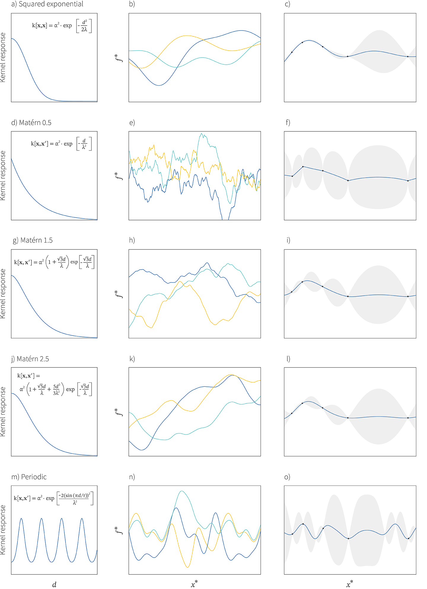
Figure 8. GP Kernels. a) Squared exponential function of distance. b) Samples from squared exponential prior. c) Squared exponential model fit to data. d-f) Matérn kernel with $\nu=0.5$. Notice that the samples are irregular and that the fit is not smooth. g-i) Matérn kernel with $\nu=1.5$. The samples are more regular and the fit is smoother j-l) Matérn kernel with $\nu=2.5$. The samples are more regular yet and the fit very smooth. m-o) Periodic kernel. The samples are periodic and the fit similarly periodic.
Periodic Kernel: If we believe that the underlying function is oscillatory, we use the periodic function:
\begin{equation}\mbox{k}[\mathbf{x},\mathbf{x}^\prime] = \alpha^{2} \cdot \exp \left[ \frac{-2(\sin[\pi d/\tau])^{2}}{\lambda^2} \right], \tag{20}\end{equation}
where $\tau$ is the period of the oscillation and the other parameters have the same meanings as before.
Learning GP parameters
A common application for Bayesian optimization is to search for the best hyperparameters of a machine learning model. However, in an ironic twist, the kernel functions used in Bayesian optimization themselves contain unknown hyper-hyperparameters like the amplitude $\alpha$, length scale $\lambda$ and noise $\sigma^{2}_{n}$. There are several possible approaches to choosing these hyperparameters:
1. Maximum likelihood: similar to training ML models, we can choose these parameters by maximizing the marginal likelihood (i.e., the likelihood of the data after marginalizing over the possible values of the function):
\begin{eqnarray}\label{eq:bo_learning} Pr(\mathbf{y}|\mathbf{x},\boldsymbol\theta)&=&\int Pr(\mathbf{y}|\mathbf{f},\mathbf{x},\boldsymbol\theta)d\mathbf{f}\nonumber\\
&=& \mbox{Norm}_{y}[\mathbf{0}, \mathbf{K}[\mathbf{X},\mathbf{X}]+\sigma^{2}_{n}\mathbf{I}], \tag{21}
\end{eqnarray}
where $\boldsymbol\theta$ contains the unknown parameters in the kernel function and the measurement noise $\sigma^{2}_{n}$.
In Bayesian optimization, we are collecting the observations sequentially, and where we collect them will depend on the kernel parameters, and we would have to interleave the processes of acquiring new points and optimizing the kernel parameters.
2. Full Bayesian approach: here we would choose a prior distribution $Pr(\boldsymbol\theta)$ on the kernel parameters of the Gaussian process and combine this with the likelihood in equation 21 to compute the posterior. We then weight the acquisition functions according to this posterior:
\begin{equation}\label{eq:snoek_post} \hat{a}[\mathbf{x}^{*}]\propto \int a[\mathbf{x}^{*}|\boldsymbol\theta]Pr(\mathbf{y}|\mathbf{x},\boldsymbol\theta)Pr(\boldsymbol\theta). \tag{22} \end{equation}
In practice this would usually be done using an Monte Carlo approach in which the posterior is represented by a set of samples (see Snoek et al., 2012) and we sum together multiple acquisition functions derived from these kernel parameter samples (figure 9).
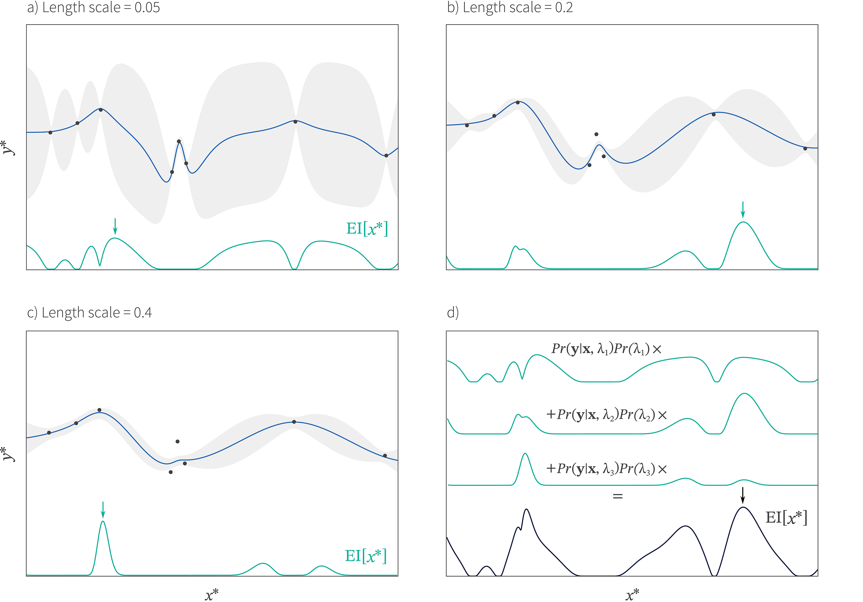
Figure 9. Bayesian approach for handling length scale of kernel from Snoek et al., 2012. a-c) We fit the model with three different length scales and compute the acquisition function for each. d) We compute a weighted sum of these acquisition functions (black curve) where the weight is given by posterior probability of the data at each scale (see equation 22). We choose the next point by finding the maximum of this weighted function (black arrow). In this way, we approximately marginalize out the length scale.
Parallel Bayesian optimization
For practical applications like hyperparameter search, we would want to make multiple function evaluations in parallel. In this case, we must consider how to prevent the algorithm from starting a new function evaluation in a place that is already being explored by a parallel thread.
One solution is to use a stochastic acquisition function. For example, Thompson sampling draws from the posterior distribution over the function and samples where this sample is maximal (figure 4d). When we sample several times, we will get different draws from the posterior and hence different values of $\mathbf{x}$.
A more sophisticated approach is to treat the problem in a fully Bayesian way (Snoek et al., 2012). The optimization algorithm keeps track of both the points that have been evaluated and the points that are pending, marginalizing over the uncertainty in the pending points. This can be done using a sampling approach similar to the method in figure 9 for incorporating different length scales. We draw samples from the Gaussians representing the possible pending results and build an acquisition function for each. We then average together these acquisition functions weighted by the probability of observing those results.
Tips, tricks, and limitations
In practice, Bayesian optimization with Gaussian Processes works best if we start with a number of points from the function that have already been evaluated. A rule of thumb might be to use random sampling for $\sqrt{d}$ iterations where $d$ is the number of dimensions and then start the Bayesian optimization process. A second useful trick is to occasionally incorporate a random sample into the scheme. This can stop the Bayesian optimization process getting waylaid examining unproductive regions of the space and forces a certain degree of exploration. A typical approach might be to use a random sample every 10 iterations.
The main limitation of Bayesian optimization with GPs is efficiency. As the dimensionality increases, more points need to be evaluated. Unfortunately, the cost of exact inference in the Gaussian process scales as $\mathcal{O}[n^3]$ where $n$ is the number of data points. There has been some work to reduce this cost through different approximations such as:
- Inducing points: This approach tries to summarize the large number of observed points into a smaller subset known as inducing points (Snelson et al., 2006).
- Decomposing the kernel: This approach decomposes the “big” kernel in high dimension into “small” kernels that act on small dimensions (Duvenaud et al., 2011).
- Using random projections: This approach relies on random embedding to solve the optimization problem in a lower dimension (Wang et al., 2013).
Discrete variables
So far, we have considered optimizing continuous variables. What does Bayesian optimization look like in the discrete case? Perhaps we wish to choose which of $K$ discrete conditions (parameter values) yields the best output. In the absence of noise, this problem is trivial; we simply try all $K$ conditions in turn and choose the one that returns the maximum. However, when there is noise on the output, we can use Bayesian optimization to find the best condition efficiently.
The basic approach is model each condition independently. For continuous observations, we could model each output $f_{k}$ with a normal distribution, choose a prior over the mean of the normal and then use the measurements to compute a posterior over this mean. We’ll leave developing this model as an exercise for the reader. Instead and for a bit of variety, we’ll move to a different setting where the observations are binary we wish to find the configuration that produces the highest proportion of ‘1’s in the output. This setting motivates the Beta-Bernoulli bandit model.
Beta-Bernoulli bandit
Consider the problem of choosing which of $K$ graphics to present to the user for a web-advert. We assume that for the $k^{th}$ graphic, there is a fixed probability $f_{k}$ that the person will click, but these parameters are unknown. We would like to efficiently choose the graphic that prompts the most clicks.
To solve this problem, we treat the parameters $f_{1}\ldots f_{K}$ as uncertain and place an uninformative Beta distribution prior with $\alpha,\beta=1$ over their values:
\begin{equation} Pr(f_{k}) = \mbox{Beta}_{f_{k}}\left[1.0, 1.0\right]. \tag{23}\end{equation}
The likelihood of showing the $k^{th}$ graphic $n_{k}$ times and receiving $c_{k}$ clicks is then
\begin{equation} Pr(c_{k}|f, n_{k}) = f_{k}^{c_{k}}(1-f_{k})^{n_{k}-c_{k}}, \tag{24}\end{equation}
and we can combine these two equations via Bayes rule to compute the posterior distribution over the parameter $f_{k}$ (see chapter 4 of Prince, 2012) which will be given by
\begin{equation} Pr(f_{k}|c_{k},n_{k}) = \mbox{Beta}_{f_{k}}\left[1.0 + c_{k}, 1.0 + n_{k}-c_{k} \right]. \tag{25} \end{equation}
Now we must choose which value of $k$ to try next given the $k$ posterior distributions over the probabilities $f_{k}$ of getting a click (figure 10). As before, we choose an acquisition function and sample the value of $k$ that maximizes this. In this case, the most practical approach is to use Thompson sampling. We sample from each posterior distribution separately (they are independent) and choose $k$ based on the highest sampled value.
As in the continuous case, this method will trade off exploiting existing knowledge by showing graphics that it knows will generate a high rate of clicks and exploring graphics where the click rate is very uncertain. This model and algorithm are part of a more general literature on bandit algorithms. More information can be found in this book.
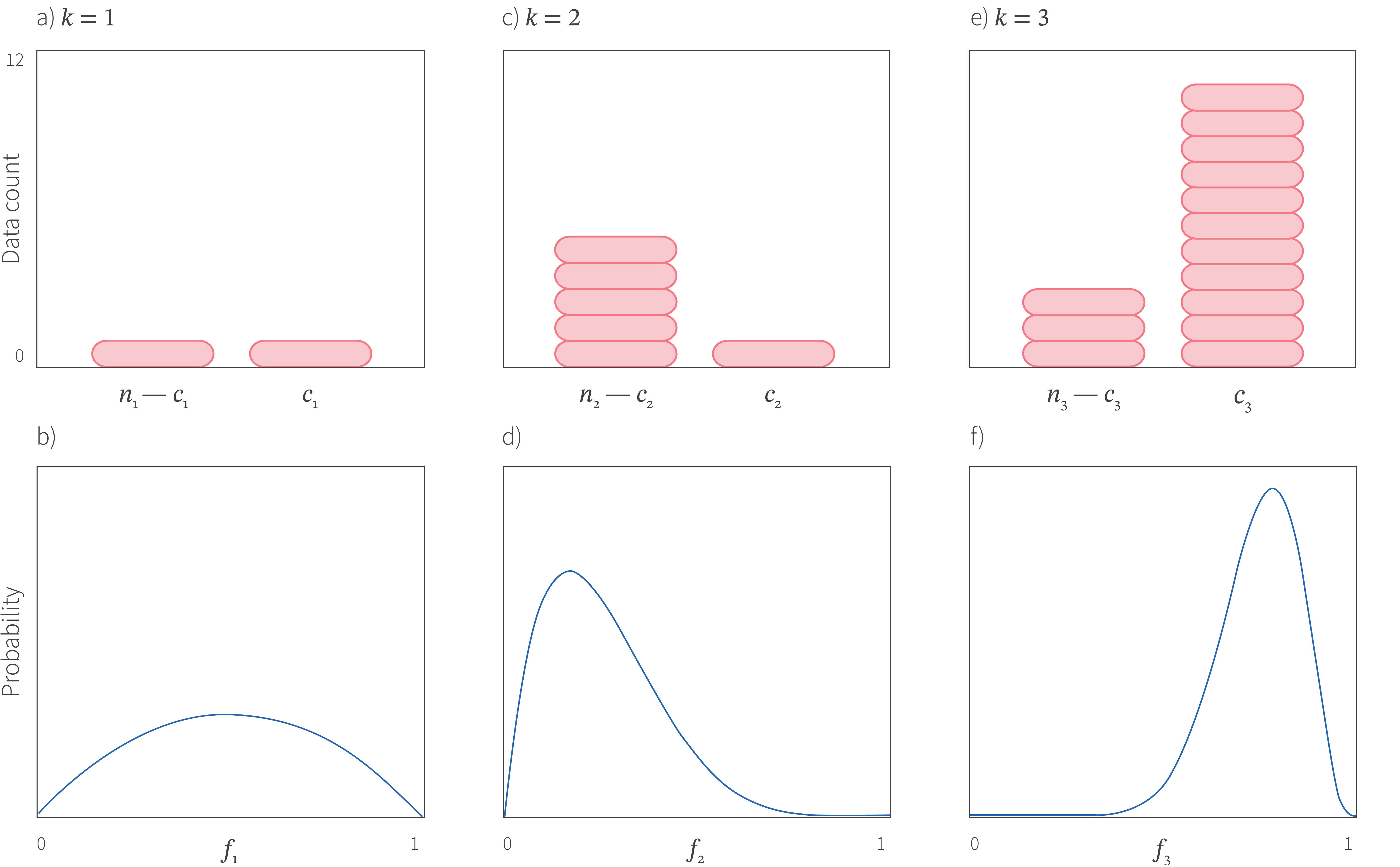
Figure 10. Beta-Bernoulli bandit with $K=3$ conditions. a) Observed data for condition $k=1$ which has been tried $n_{1}=2$ times with $c_{1}=1$ success. b) Consequently, the value for the parameter $f_{1}$ representing the probability of success is very uncertain. We know for sure that it cannot be zero or one but all other values are plausible. c) In condition $k=2$ we have seen 1 success out of 6. d) The posterior over the parameter $f_{2}$ is peaked at lower values. e) For condition $k=3$ we have seen 11 successes out of 14. f) Here the posterior is even more peaked and at high values representing the fact that we have mostly seen successes. For Thompson sampling, we would pick one sample each from the three posteriors in panels b,d, and f and choose the condition where the sample takes the greatest value. This will mostly tend to choose condition $k=3$ (exploiting the best choice we have seen so far) or condition 1 (exploring the most uncertain condition).
Multiple discrete variables
When we have many discrete variables (e.g., the orientation, color, font size in an advert graphic), we could treat each combination of variables as one value of $k$ and use the above approach in which each condition is treated independently. However, the number of combinations may be very large and so this is not necessarily practical.
If the discrete variables have a natural order (e.g., font size) then one approach is to treat them as continuous. We amalgamate them into an observation vector $\mathbf{x}$ and use a Gaussian process model. The only complication is that we now only compute the acquisition function at the discrete values that are valid.
If the discrete variables have no natural order then we are in trouble. Gaussian processes depend on the kernel ‘distance’ between points and it is hard to define such kernels for discrete variables. One approach is to use a one-hot encoding, apply a kernel for each dimension and let the overall kernel be defined by the product of these sub-kernels (Duvenaud et al., 2014). However, this is not ideal because there is no way for the model to know about the invalid input values which will be assigned some probability and may be selected as new points to evaluate. One way to move forward is to consider a different underling probabilistic model.
Different probabilistic models
The approaches up to this point can deal with most of the problems that we outline in the introduction, but are not suited to the case where there are many discrete variables (possibly in combination with continuous variables). Moreover, they cannot elegantly handle the case of conditional variables where the existence of some variables is contingent on the settings of others. In this section we consider random forest models and tree-Parzen estimators, both of which can handle these situations.
Random forests
The Sequential Model-based Algorithm Configuration (SMAC) algorithm uses a random forest as an alternative to Gaussian processes. Consider the case where we have made some observations and trained a regression forest. For any point, we can measure the mean of the trees’ predictions and their variance (figure 11). This mean and variance are then treated similarly to the equivalent outputs from a Gaussian process model. We apply an acquisition function to choose which of a set of candidate points to sample next. In practice, the forest must be updated as we go along and a simple way to do that is just to split a leaf when it accumulates a certain number of training examples.
Random forests based on binary splits can easily cope with combinations of discrete and continuous variables; it is just as easy to split the data by thresholding a continuous value as it is to split it by dividing a discrete variable into two non-overlapping sets. Moreover, the tree structure makes it easy to accommodate conditional parameters: we do not consider splitting on contingent variables until they are guaranteed by prior choices to exist.

Figure 11. Sequential Model-based Algorithm Configuration (SMAC) algorithm. Here the Gaussian process model is replaced by a regression forest. a) Output of first tree, which has split first at position $x_{1}$ and then the left and right branch have themselves split at positions $x_{11}$ and $x_{12}$ respectively, to result in four leaves, each of which takes a different value. b-c) Two more trees that model the data slightly differently by splitting in different places. d) For each position $x^{*}$ we now have three possible values from the three trees. We compute the mean and variance of these values to make a model representing the mean and uncertainty of the underlying function.
Tree-Parzen estimators
The Tree-Parzen estimator (Bergstra et al., 2011) works quite differently from the models that we have considered so far. It describes the likelihood $Pr(\mathbf{x}|y)$ of the data $\mathbf{x}$ given the noisy function value $y$ rather than the posterior $Pr(y|\mathbf{x})$.
More specifically, the goal is to build two separate models $Pr(\mathbf{x}|y\in\mathcal{L})$ and $Pr(\mathbf{x}|y\in\mathcal{H})$ where the set $\mathcal{L}$ contains the lowest values of $y$ seen so far and the set $\mathcal{H}$ contains the highest. These sets are created by partitioning the values according to whether they fall below or above some fixed quantile.
The likelihoods $Pr(\mathbf{x}|y\in\mathcal{L})$ and $Pr(\mathbf{x}|y\in\mathcal{H})$ are modelled with kernel density estimators; for example, we might describe the likelihood as a sum of Gaussians with a mean on each observed data point $\mathbf{x}$ and fixed variance (figure 12). It can be shown that expected improvement is then maximized by choosing the point that maximizes the ratio $Pr(\mathbf{x}|y\in\mathcal{H})/Pr(\mathbf{x}|y\in\mathcal{L})$.
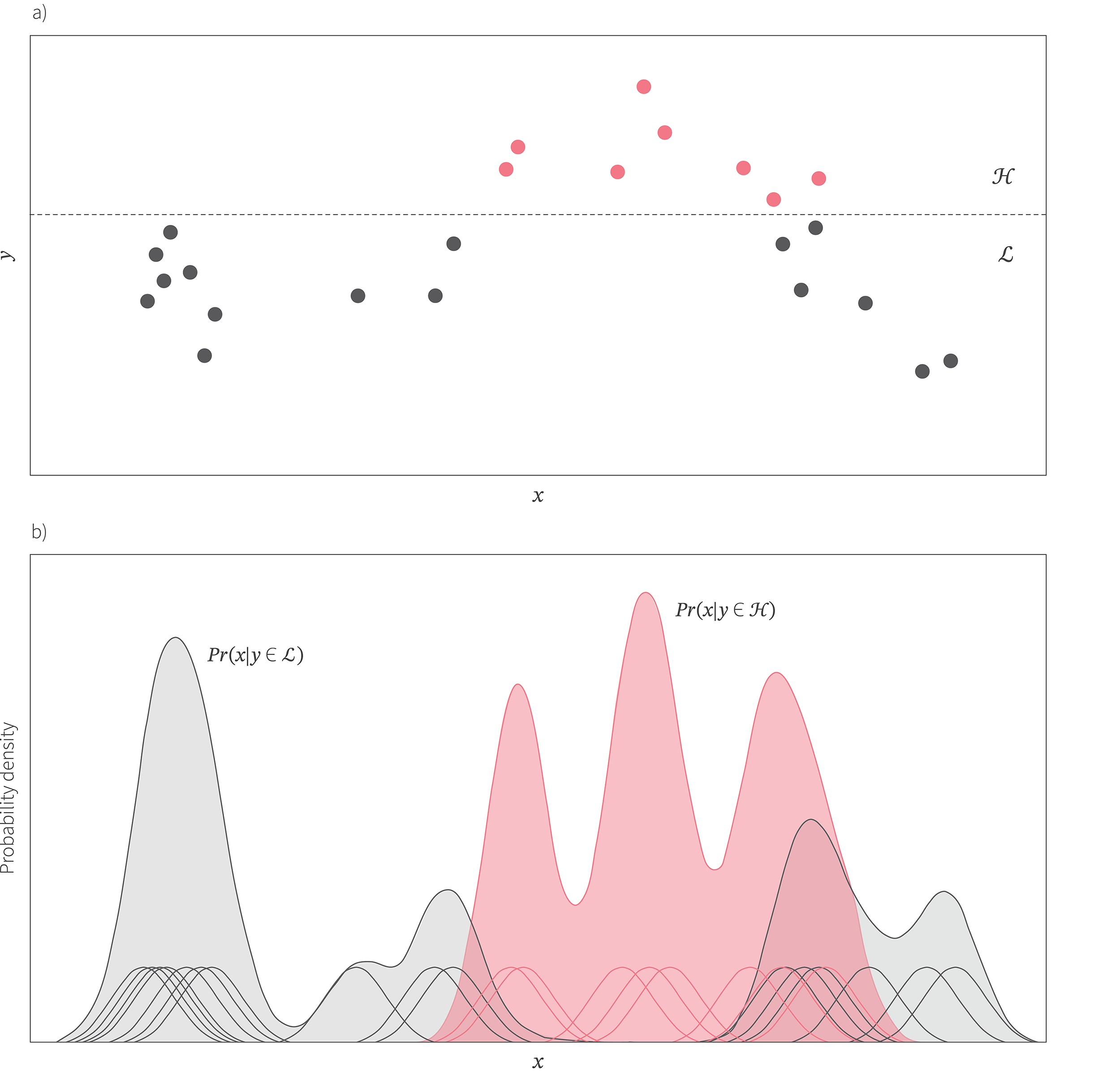
Figure 12. Tree-Parzen estimators. a) Tree-Parzen estimators divide the data into two sets $\mathcal{L}$ and $\mathcal{H}$ by thresholding the observed function values. b) They then build a probability density of each set using a Parzen kernel estimator — they place a Gaussian at each data point and sum these Gaussians to get the final data distribution. A point is desirable to sample next if the probability $Pr(x|y\in \mathcal{H})$ of being in the set $\mathcal{H}$ of high-values is large and the probability $Pr(x|y\in \mathcal{L})$ of being in the set $\mathcal{L}$ is low.
Tree-Parzen estimators work when we have a mixture of discrete and continuous spaces, and when some parameters are contingent on others. Moreover, the computation scales linearly with the number of data points as opposed to with their cube as for Gaussian processes.
Further information
In this tutorial, we have discussed Bayesian optimization, its key components, and applications. For further information, consult the recent surveys by Shahriari et al. (2016) and Frazier 2018. Python packages for Bayesian optimization include BoTorch, Spearmint, GPFlow, and GPyOpt.
Code for hyperparameter optimization can be found in the Hyperopt and HPBandSter packages. A popular application of Bayesian optimization is for AutoML which broadens the scope of hyperparameter optimization to also compare different model types as well as choosing their parameters and hyperparameters. Python packages for AutoML include Auto-sklearn, Hyperop-sklearn, and NNI.
Work with Us!
Impressed by the work of the team? RBC Borealis is looking to hire for various roles across different teams. Visit our career page now and discover opportunities to join similar impactful projects!
Careers at RBC Borealis