
Introduction
This tutorial concerns the Boolean satisfiability or SAT problem. We are given a formula containing binary variables that are connected by logical relations such as $\text{OR}$ and $\text{AND}$. We aim to establish whether there is any way to set these variables so that the formula evaluates to $\text{true}$. Algorithms that are applied to this problem are known as SAT solvers.
The tutorial is divided into three parts. In part I, we introduce Boolean logic and the SAT problem. We discuss how to transform SAT problems into a standard form that is amenable to algorithmic manipulation. We categorize types of SAT solvers and present two naïve algorithms. We introduce several SAT constructions, which can be thought of as common sub-routines for SAT problems. Finally, we present some applications; the Boolean satisfiability problem may seem abstract, but as we shall see it has many practical uses.
In part II of the tutorial, we will dig more deeply into the internals of modern SAT solver algorithms. In part III, we recast SAT solving in terms of message passing on factor graphs. We also discuss satisfiability modulo theory (SMT) solvers, which extend the machinery of SAT solvers to solve more general problems involving continuous variables.
Relevance to machine learning
The relevance of SAT solvers to machine learning is not immediately obvious. However, there are two direct connections. First, machine learning algorithms rely on optimization. SAT can also be considered an optimization problem and SAT solvers can find global optima without relying on gradients. Indeed, in this tutorial, we’ll show how to fit both neural networks and decision trees using SAT solvers.
Second, machine learning techniques are often used as components of SAT solvers; in part II of this tutorial, we’ll discuss how reinforcement learning can be used to speed up SAT solving, and in part III we will show that there is a close connection between factor graphs and SAT solvers and that belief propagation algorithms can be used to solve satisfiability problems.
Boolean logic and satisfiability
In this section, we define a set of Boolean operators and show how they are combined into Boolean logic formulae. Then we introduce the Boolean satisfiability problem.
Boolean operators
Boolean operators are standard functions that take one or more binary variables as input and return a single binary output. Hence, they can be defined by truth tables in which we enumerate every combination of inputs and define the output for each (figure 1). Common logical operators include:
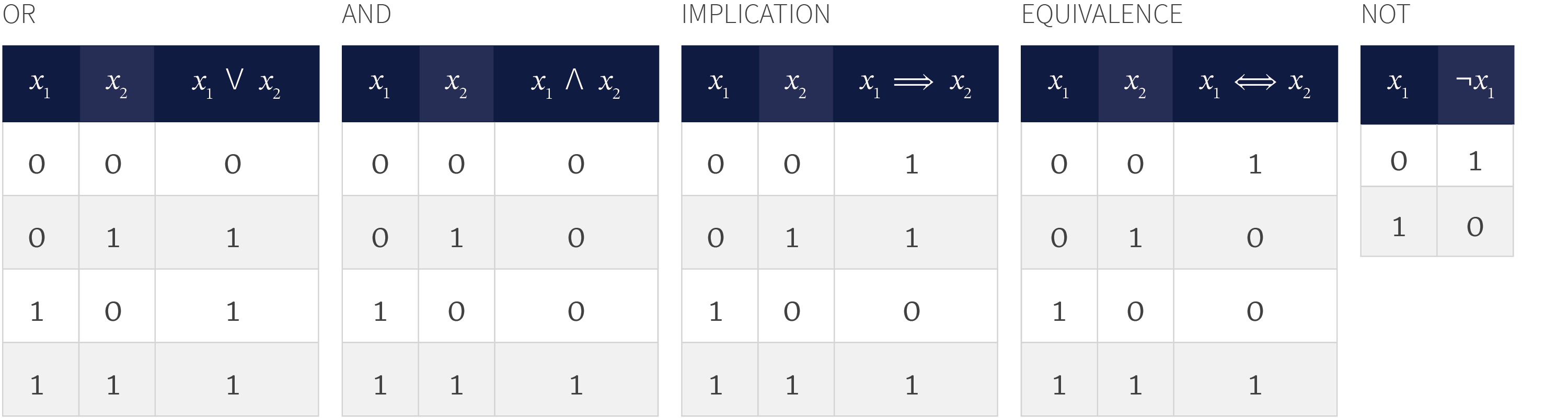
Figure 1. Logical operators. Each of the first four operators ($\text{OR}$, $\text{AND}$, $\text{IMPLICATION}$and $\text{EQUIVALENCE}$) takes two binary input variables $x_{1}$ and $x_{2}$ and returns either $\text{true}$ or $\text{false}$ (shown here as 1 and 0). The $\text{NOT}$ operator takes a single binary input returns its complement.
- The $\text{OR}$ operator is written as $\lor$ and takes two inputs $x_{1}$ and $x_{2}$. It returns $\text{true}$ if one or both of the inputs are $\text{true}$ and returns $\text{false}$ otherwise.
- The $\text{AND}$ operator is written as $\land$ and takes two inputs $x_{1}$ and $x_{2}$. It returns $\text{true}$ if both the inputs are $\text{true}$ and $\text{false}$ otherwise.
- The $\text{IMPLICATION}$ operator is written as $\Rightarrow$ and evaluates whether the two inputs are consistent with the statement ‘if $x_{1}$ then $x_{2}$’. The statement is only disobeyed when $x_{1}$ is $\text{true}$ and $x_{2}$ is $\text{false}$ and so implication returns $\text{false}$ for this combination of inputs and $\text{true}$ otherwise.
- The $\text{EQUIVALENCE}$ operator is written as $\Leftrightarrow$ and takes two inputs $x_{1}$ and $x_{2}$. It returns $\text{true}$ if the two inputs are the same and returns $\text{false}$ otherwise.
- The $\text{NOT}$ operator is written as $\lnot$ and takes one input. It returns $\text{true}$ if the input $x_{1}$ is $\text{false}$ and vice-versa. We refer $\lnot x_{1}$ as the complement of $x_{1}$.
Boolean logic formulae
A Boolean logic formula $\phi$ takes a set of $I$ variables $\{x_{i}\}_{i=1}^{I}\in\{$$\text{false}$,$\text{true}$$\}$ and combines them using Boolean operators, returning $\text{true}$ or $\text{false}$. For example:
\begin{equation} \phi:= (x_{1}\Rightarrow (\lnot x_{2}\land x_{3})) \land (x_{2} \Leftrightarrow (\lnot x_{3} \lor x_{1}). \tag{1}\end{equation}
For any combination of input variables $x_{1},x_{2},x_{3}\in\{$$\text{false}$,$\text{true}$$\}$, we could evaluate this formula and see if it returns $\text{true}$ or $\text{false}$. Notice that even for this simple example with three variables it is hard to see what the answer will be by inspection.
Boolean satisfiability and SAT solvers
The Boolean satisfiability problem asks whether there is at least one combination of binary input variables $x_{i}\in\{$$\text{false}$,$\text{true}$$\}$ for which a Boolean logic formula returns $\text{true}$. When this is the case, we say the formula is satisfiable.
A SAT solver is an algorithm for establishing satisfiability. It takes the Boolean logic formula as input and returns $\text{SAT}$ if it finds a combination of variables that can satisfy it or $\text{UNSAT}$ if it can demonstrate that no such combination exists. In addition, it may sometimes return without an answer if it cannot determine whether the problem is $\text{SAT}$ or $\text{UNSAT}$.
Conjunctive normal form
To solve the SAT problem, we first convert the Boolean logic formula to a standard form that it is more amenable to algorithmic manipulation. Any formula can be re-written as a conjunction of disjunctions (i.e., the logical $\text{AND}$ of statements containing $\text{OR}$ relations). This is known as conjunctive normal form. For example:
\begin{equation}\label{eq:example_cnf} \phi:= (x_{1} \lor x_{2} \lor x_{3}) \land (\lnot x_{1} \lor x_{2} \lor x_{3}) \land (x_{1} \lor \lnot x_{2} \lor x_{3}) \land (x_{1} \lor x_{2} \lor \lnot x_{3}). \tag{2}\end{equation}
Each term in brackets is known as a clause and combines together variables and their complements with a series of logical $\text{OR}$s. The clauses themselves are combined via $\text{AND}$ relations.
The Tseitin transformation
The Tseitin transformation converts an arbitrary logic formula to conjunctive normal form. The approach is to i) associate new variables with sub-parts of the formula using logical equivalence relations, (ii) to restate the formula by logically $\text{AND}$-ing these new variables together, and finally (iii) manipulate each of the equivalence relations so that they themselves are in conjunctive normal form.
This process is most easily understood with a concrete example. Consider the conversion of the formula:
\begin{equation}
\phi:= ( (x_{1} \lor x_{2}) \Leftrightarrow x_{3})\Rightarrow (\lnot x_{4}). \tag{3}
\end{equation}
Step 1: We associate new binary variables $y_{i}$ with the sub-parts of the original formula using the $\text{EQUIVALENCE}$ operator:
\begin{eqnarray}\label{eq:tseitin}
y_{1} &\Leftrightarrow &(x_{1} \lor x_{2})\nonumber \
y_{2} &\Leftrightarrow &(y_{1} \Leftrightarrow x_{3}) \nonumber \
y_{3} &\Leftrightarrow &\lnot x_{4}\nonumber \
y_{4} &\Leftrightarrow &(y_{2} \Rightarrow y_{3}). \tag{4}
\end{eqnarray}
We work from the inside out (i.e., from the deepest brackets to the least deep) and choose sub-formulae that contain a single operator ($\lor, \land, \lnot, \Rightarrow$ or $\Leftrightarrow$).
Step 2: We restate the formula in terms of these relations. The full original statement is now represented by $y_{4}$ together with the definitions of $y_{1},y_{2},y_{3},y_{4}$ in equations 4. So the statement is $\text{true}$ when we combine all of these relations with logical $\text{AND}$ relations. Working backwards we get:
\begin{eqnarray}\label{eq:tseitin_stage2}
\phi&=& y_{4} \land (y_{4} \Leftrightarrow (y_{2} \Rightarrow y_{3})) \nonumber \\&&\hspace{0.4cm}\land (y_{3} \Leftrightarrow \lnot x_{4})\nonumber \\&& \hspace{0.4cm}\land (y_{2} \Leftrightarrow (y_{1} \Leftrightarrow x_{3}))\nonumber
\\&&\hspace{0.4cm}\land (y_{1} \Leftrightarrow (x_{1} \lor x_{2})). \tag{5}
\end{eqnarray}
This is getting closer to the conjunctive normal form as it is now a conjunction (logical $\text{AND}$) of different terms.
Step 3: We convert each of these individual terms to conjunctive normal form. In practice, there is a recipe for each type of operator:
\begin{eqnarray}a \Leftrightarrow (\lnot b) & = & (a \lor b) \land (\lnot a \lor \lnot b) \\a \Leftrightarrow (b \lor c) &= & (a\lor \lnot b) \land (a \lor \lnot c) \land (\lnot a \lor b \lor c) \nonumber \\a \Leftrightarrow (b \land c) & = & (\lnot a \lor b) \land (\lnot a \lor c) \land (a \lor \lnot b \lor \lnot c) \nonumber \\a \Leftrightarrow (b \Rightarrow c) & = & (a \lor b) \land (a \lor \lnot c) \land (\lnot a \lor \lnot b \lor c) \nonumber \\a \Leftrightarrow (b \Leftrightarrow c) & = & (\lnot a \lor \lnot b \lor c)\land (\lnot a \lor b \lor \lnot c) \land (a \lor \lnot b \lor \lnot c) \land (a\lor b\lor c).\nonumber \tag{6}\end{eqnarray}
The first of these recipes is easy to understand. If $a$ is $\text{true}$ then the first clause is satisfied, but the second can only be satisfied by having $\lnot b$. If $a$ is $\text{false}$ then the second clause is satisfied, but the first clause can only be satisfied by $b$. Hence when $a$ is $\text{true}$, $\lnot b$ is $\text{true}$ and when $a$ is $\text{false}$, $\lnot b$ is $\text{false}$ and so $a \Leftrightarrow (\lnot b)$ as required.
The remaining recipes are not obvious, but you can confirm that they are correct by writing out the truth tables for the left and right sides of each expression and confirming that they are the same. Applying the recipes to equation 5 we get the final expression in conjunctive normal form:
\begin{eqnarray}\label{eq:tseitin_stage3}\phi\!\!&\!\!:=& y_{4} \land (y_4\lor y_2) \land (y_4 \lor \lnot y_3) \land (\lnot y_4 \lor \lnot y_2 \lor y_3)\nonumber \\&&\hspace{0.4cm}\land (y_3 \lor x_4) \land (\lnot y_3 \lor \lnot x_4)\nonumber\\&& \hspace{0.4cm}\land (\lnot y_2 \lor \lnot y_1 \lor x_3)\land (\lnot y_2 \lor y_1 \lor \lnot x_3) \land (y_2 \lor \lnot y_1 \lor \lnot x_3) \land (y_2\lor y_1\lor x_3)\nonumber \\&&\hspace{0.4cm}\land (y_1\lor \lnot x_1) \land (y_1 \lor \lnot x_2) \land (\lnot y_1 \lor x_1 \lor x_2). \tag{7}\end{eqnarray}
Literals
In the conjunctive normal form, each clause is a disjunction (logical $\text{OR}$) of variables and their complements. For neatness, we will write the complement $\lnot x$ of a variable as $\overline{x}$, so instead of writing:
\begin{equation} \phi:= (x_{1} \lor x_{2} \lor x_{3}) \land (\lnot x_{1} \lor x_{2} \lor x_{3}) \land (x_{1} \lor \lnot x_{2} \lor x_{3}) \land (x_{1} \lor x_{2} \lor \lnot x_{3}), \tag{8}\end{equation}
we write:
\begin{equation}\label{eq:example_cnf2} \phi:= (x_{1} \lor x_{2} \lor x_{3}) \land (\overline{x}_{1} \lor x_{2} \lor x_{3}) \land (x_{1} \lor \overline{x}_{2} \lor x_{3}) \land (x_{1} \lor x_{2} \lor \overline{x}_{3}). \tag{9}\end{equation}
We collectively refer to the variables and their complements as literals and so this formula contains literals $x_{1},\overline{x}_{1},x_{2},\overline{x}_{2}, x_{3}$ and $\overline{x}_{3}.$
$k$-clauses and $k$-SAT
When expressed in conjunctive normal form, we can characterise the problem in terms of the number of variables, the number of clauses and the size of those clauses. To facilitate this we introduce the following terminology:
- A clause that contains kk variables is known as a kk-clause. When a clause contains only a single variable, it is known as a unit clause.
- When all the clauses contain kk variables, we refer to a problem as kk-SAT. Using this nomenclature, we see that equation 9 is a 3-SAT problem.
Establishing satisfiability
SAT solvers are algorithms that establish whether a Boolean expression is satisfiable and they can be classified into two types. Complete algorithms guarantee to return $\text{SAT}$ or $\text{UNSAT}$ (although they may take an impractically long time to do so). Incomplete algorithms return $\text{SAT}$ or return $\text{UNKNOWN}$ (i.e. return without providing an answer). If they find a solution that satisfies the expression then all is good, but if they don’t then we can draw no conclusions.
Here are two naïve algorithms that will help you understand the difference:
- An example of a complete algorithm is exhaustive search. If there are VV variables, we evaluate the expression with all 2V2V combinations of literals and see if any combination returns truetrue. Obviously, this will take an impractically long time when the number of variables are large, but nonetheless it is guaranteed to return either SATSAT or UNSATUNSAT eventually.
- An example of an incomplete algorithm is Schöning’s random walk. This is a Monte Carlo solver in which we repeatedly (i) randomly choose an unsatisfied clause, (ii) choose one of the variables in this clause at random and set it to the opposite value. At each step we test if the formula is now satisfied and if so return SATSAT. After 3V3V iterations, we return UNKNOWNUNKNOWN if we have not found a satisfying configuration.
When a solver returns $\text{SAT}$ or $\text{UNSAT}$, it also returns a certificate, which can be used to check the result with a simpler algorithm. If the solver returns $\text{SAT}$, then the certificate will be a set of variables that obey the formula. These can obviously be checked by simply computing the formula with them and checking that it returns $\text{true}$ . If it returns $\text{UNSAT}$ then the certificate will usually be a complex data structure that depends on the solver.
Bad news and good news
First, the bad news. The SAT problem is proven to be NP-complete and it follows that there is no known polynomial algorithm for establishing satisfiability in the general case. An important exception to this statement is 2-SAT for which a polynomial algorithm is known. However, for 3-SAT and above the problem is very difficult.
The good news is that modern SAT solvers are very efficient and can often solve problems involving tens of thousands of variables and millions of clauses in practice. In part II of this tutorial we will explain how these algorithms work.
Related problems to SAT
Until now we have focused on the satisfiability problem in which we try to establish if there is at least one set of literals that makes a given statement evaluate to $\text{true}$. We note that there are also a number of closely related problems:
UNSAT: In the UNSAT problem we aim to show that there is no combination of literals that satisfies the formula. This is subtly different from SAT where algorithms return as soon as they find literals that show the formula is $\text{SAT}$, but may take exponential time if they cannot find a solution. For the UNSAT problem, the converse is true. The algorithm will return as soon as soon as it establishes the formula is not $\text{UNSAT}$, but may take exponential time to show that it is $\text{UNSAT}$.
Model counting: In model counting (sometimes referred to as #SAT or #CSP), our goal is to count the number of distinct sets of literals that satisfy the formula.
Max-SAT: In Max-SAT, it may be the case that a formula is $\text{UNSAT}$ but we aim to find a solution that minimizes the number of clauses that are invalid.
Weighted Max-SAT: This is a variation of Max-SAT in which we pay a different penalty for each clause when it is invalid. We wish to find the solution that incurs the least penalty.
For the rest of this tutorial, we’ll concentrate on the main SAT problem, but we’ll return to these related problems in part III of this tutorial when we discuss factor graph methods.
SAT Constructions
Most of the remainder of part I of this tutorial is devoted to discussing practical applications of satisfiability problems. Based on the discussion thus far, the reader would be forgiven for being sceptical about how this rather abstract problem can find real-world uses. We will attempt to convince you that it can! However, before we can do this, it will be helpful to review commonly-used SAT constructions.
SAT constructions can be thought of as subroutines for Boolean logic expressions. A common situation is that we have a set of variables $x_{1},x_{2},x_{3},\ldots$ and we want to enforce a collective constraint on their values. In this section, we’ll discuss how to enforce the constraints that they are all the same, that exactly one of them is $\text{true}$, that no more than $K$ of them are true or that exactly $K$ of them are true.
Same
To enforce the constraint that a set of variables $x_{1},x_{2}$ and $x_{3}$ are either all $\text{true}$ or all $\text{false}$ we simply take the logical $\text{OR}$ of these two cases so we have:
\begin{equation} \mbox{Same}[x_{1},x_{2},x_{3}]:= (x_{1}\land x_{2}\land x_{3})\lor(\overline{x}_{1}\land \overline{x}_{2}\land \overline{x}_{3}). \tag{10}\end{equation}
Note that this is not in conjunctive normal form (the $\text{AND}$ and $\text{OR}$s are the wrong way around) but could be converted via the Tseitin transformation.
Exactly one
To enforce the constraint that only one of a set of variables $x_{1},x_{2}$ and $x_{3}$ is true and the other two are false, we add two constraints. First we ensure that at least one variable is $\text{true}$ by logically $\text{OR}$ing the variables together:
\begin{equation} \phi_{1}:= x_{1}\lor x_{2} \lor x_{3}. \tag{11}\end{equation}
Then we add a constraint that indicates that both members of any pair of varaiables cannot be simultaneously $\text{true}$:
\begin{equation}\label{eq:exactly_one} \mbox{ExactlyOne}[x_{1},x_{2},x_{3}]:= \phi_{1}\land \lnot (x_{1}\land x_{2}) \land \lnot (x_{1}\land x_{3}) \land \lnot (x_{2}\land x_{3}) . \tag{12}\end{equation}
At least $K$, Less than $K$, Exactly $K$
There are many standard ways to enforce the constraint that at least $K$ of a set of variables are $\text{true}$. We’ll present one method which is a simplified version of the sequential counter encoding.
The idea is straightforward. If we have $J$ variables $x_{1},x_{2},\ldots x_{J}$ and wish to test if $K$ or more are true, we construct a $J\times K$ matrix containing new binary variables $r_{j,k}$ (figures 2b and d). The $j^{th}$ row of the table contains a count of the number of $\text{true}$ elements we have seen in $x_{1\ldots j}$. So, if we have seen 3 variables that are $\text{true}$ in the first $j$ elements, the $j^{th}$ row will start with 3 $\text{true}$ elements and finish with $K-3$ $\text{false}$ elements.
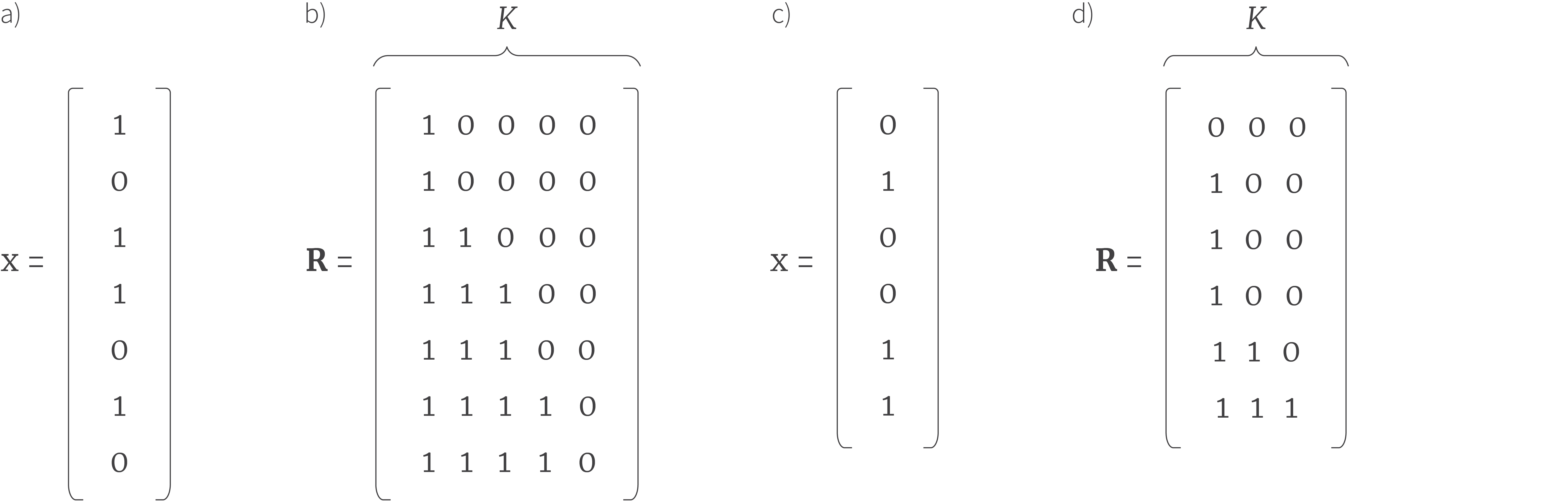
Figure 2. SAT construction for ‘at least $K$’ constraint. a) Consider a vector $\mathbf{x}$ of length 7 with elements $x_{j}$. We will show how to test whether it has at least $K=5$ elements that are $\text{true}$. b) We construct a $7\times 5$ matrix $\mathbf{R}$ where the $j^{th}$ row counts how many $\text{true}$ values we have seen up to and including the $j^{th}$ element of $\mathbf{x}$. This value is clipped if we have seen more than $K$ so far. For example, the fifth row contains 3 $\text{true}$ values (here represented as a 1) and two $\text{false}$ values (represented as a zero) indicating that there are 3 $\text{true}$ values in the first 5 elements of $\mathbf{x}$. If the ‘at least $K$’ constraint is obeyed then the bottom right element of the table will be $\text{true}$. Here, this is not the case. c) A second example vector $\mathbf{x}$ containing 6 elements. d) We construct a $6\times 3$ table to establish if there are at least 3 $\text{true}$ elements in $\mathbf{x}$. Here, that constraint is satisfied as the bottom right element is $\text{true}$.
If there are at least $K$ variables, then the bottom right variable $r_{J,K}$ in this table must be $\text{true}$ and so in practice, we would add a clause $(r_{J,K})$ stating that this bottom right element must be $\text{true}$ to enforce the constraint. When this element is $\text{false}$, the solver will search for a different solution where $\mathbf{x}$ does have at least $K$ elements or return $\text{UNSAT}$ if it cannot find one. By the same logic, to enforce the constraint that there are less than $K$ elements, we add a clause $\overline{r}_{J,K}$ stating that the bottom right hand variable is $\text{false}$.
The table in figure 2d also shows us how to constrain the data to have exactly K $\text{true}$ values. Here we would need to construct a table with $K+1$ columns. We expect the bottom right element to be $\text{false}$ (there are not K+1 $\text{true}$ values), but the element to the left of this to be $\text{true}$ (there are at least K $\text{true}$ values). Hence, we can add the clause $(\overline{r}_{J,K+1}\land r_{J,K})$. Figure 3 provides more detail about how we add extra clauses to the SAT formula that build these tables.
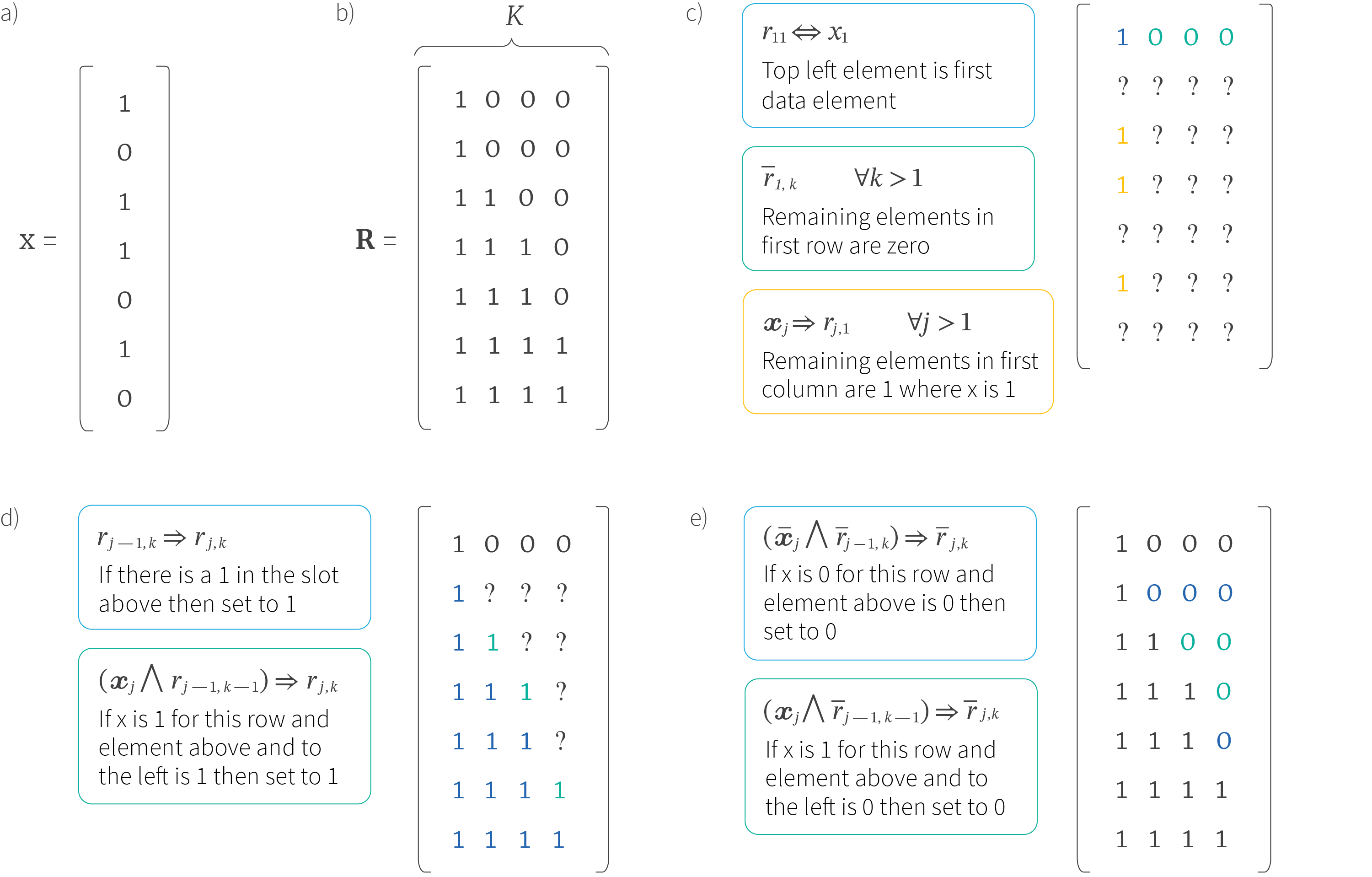
Figure 3. SAT construction for ‘at least K’ constraint. a) Consider a data vector $\mathbf{x}$ of length 7 with elements $x_{j}$. b) To test whether it has at least $K=4$ elements that are $\text{true}$, we construct a $7\times 4$ matrix $\mathbf{R}$ where the $j^{th}$ row counts how many $\text{true}$ values we have seen up to and including the $j^{th}$ element of $\mathbf{x}$. c-e) Incremental construction of the table. When we start all elements in the table are uncertain (represented by ‘?’). We $\text{AND}$ together a series of clauses that collectively constrain them to form the table. In each case, the color of the constraint matches the color of the elements it constrains.
Armed with these SAT constructions, we’ll now present two complementary ways of thinking about SAT applications. The goal is to inspire the novice reader to see the applicability to their own problems. In the next section, we’ll consider SAT in terms of constraint satisfaction problems and in the section following that, we’ll discuss it in terms of model fitting.
Applications: constraint satisfaction
The constraint satisfaction viewpoint considers combinatorial problems where there are a very large number of potential solutions, but most of those solutions are ruled out by some pre-specified constraints. To make this explicit, we’ll consider the two examples of graph coloring and scheduling.
Graph coloring
In the graph coloring problem (figure 4) we are given a graph consisting of a set of vertices and edges. We want to associate each vertex with a color in such a way that every pair of vertices connected by an edge have different colors. We might also want to know how many colors are necessary to find a valid solution. Note that this maps to our description of the generic constraint satisfaction problem; there are a large number of possible assignments of colors, but many of these are ruled out by the constraint that neighboring colors must be different.
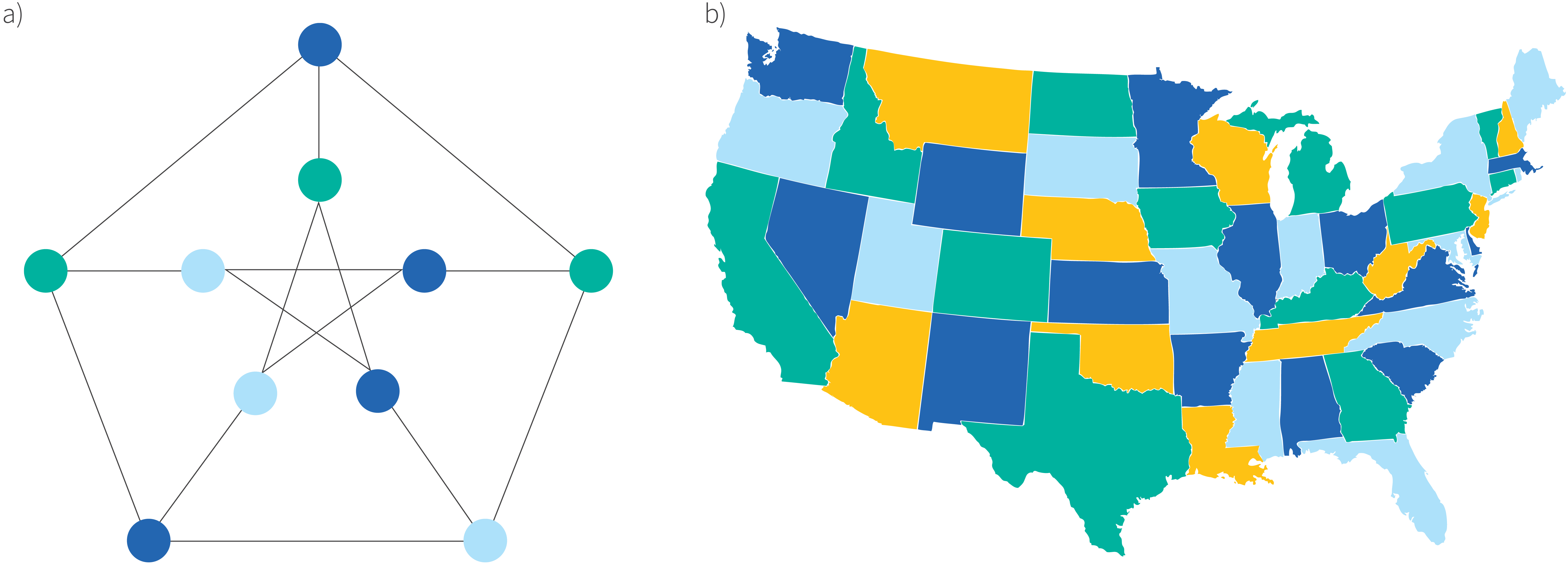
Figure 4. Graph coloring. a) We are given a graph consisting of a set of vertices and edges connecting them. We want to color the vertices in such a way that two vertices have different colors if they are connected by an edge. The graph coloring problem aims to establish the smallest number of colors for which this is possible and return a satisfying assignment of colors. For this graph, it can be achieved with three colors. b) The graph coloring problem has a practical application in coloring maps. Here each American state corresponds to a vertex and we add an edge if two states are adjacent. It has been famously proven that all such 2D maps require a maximum of four colors.
To encode this as a SAT problem, we’ll choose the number of colors $C$ to test. Then we create binary variables $x_{c,v}$ which will be $\text{true}$ if vertex $v$ is colored with color $c$. We then encode the constraint that each vertex can only have exactly one color using the construction $\mbox{ExactlyOne}[x_{\bullet, v}]$ from equation 12. We also add the constraints to ensure that the neighbours have different colors. Formally this means that that $x_{c,v}\Rightarrow \lnot x_{c,v’}$ for every color $c$ and neighbour $v’$ of vertex $v$.
Having set up the problem, we run the SAT solver. If it returns $\text{UNSAT}$ this means we need more colors. If it returns $\text{SAT}$ with a concrete coloring, then we have an answer. We can find the minimum number of colors required by using binary search over the number of colors to find the point where the problem changes from $\text{SAT}$ to $\text{UNSAT}$.
Scheduling
The graph coloring problem is a rather artificial computer science example, but many real-world problems can similarly be expressed in terms of satisfiability. For example, consider scheduling courses in a university. We have a number of professors, each of whom teach several different courses. We have a number of classrooms. We have a number of possible time-slots in each classroom. Finally, we have the students themselves, who are each signed up to a different subset of courses. We can use the SAT machinery to decide which course will be taught in which classroom and in what time-slot so that no clashes occur.
In practice, this is done by defining binary variables describing the known relations between the real world quantities. For example, we might have variables $x_{i,j}$ indicating that student $i$ takes course $j$. Then we encode the relevant constraints: no teacher can teach two classes simultaneously, no student can be in two classes simultaneously, no room can host more than one class simultaneously, and so on. The details are left as an exercise to the reader, but the similarity to the graph coloring problem is clear.
SAT as function fitting
A second way to think about satisfiability is in terms of function fitting. Here, there is a clear connection to machine learning in which we fit complex functions (i.e., models) to training data. In fact there is a simple relationship between function-fitting and constraint satisfaction; when we fit a model, we can consider the parameters as unknown variables, and each training data/label pair represents a constraint on the values those parameters can take. In this section, we’ll consider fitting binary neural networks and decision trees.
Fitting binary neural networks
Binary neural networks are nets in which both the weights and activations are binary. Their performance can be surprisingly good, and their implementation can be extremely efficient. We’ll show how to fit a binary neural network using SAT.
Following Mezard and Mora (2008) we consider a one layer binary network with $K$ neurons. The network takes a $J$ dimensional data example $\mathbf{x}$ with elements $x_{j}\in\{-1,1\}$ and computes a label $y\in\{-1,1\}$, using the function:
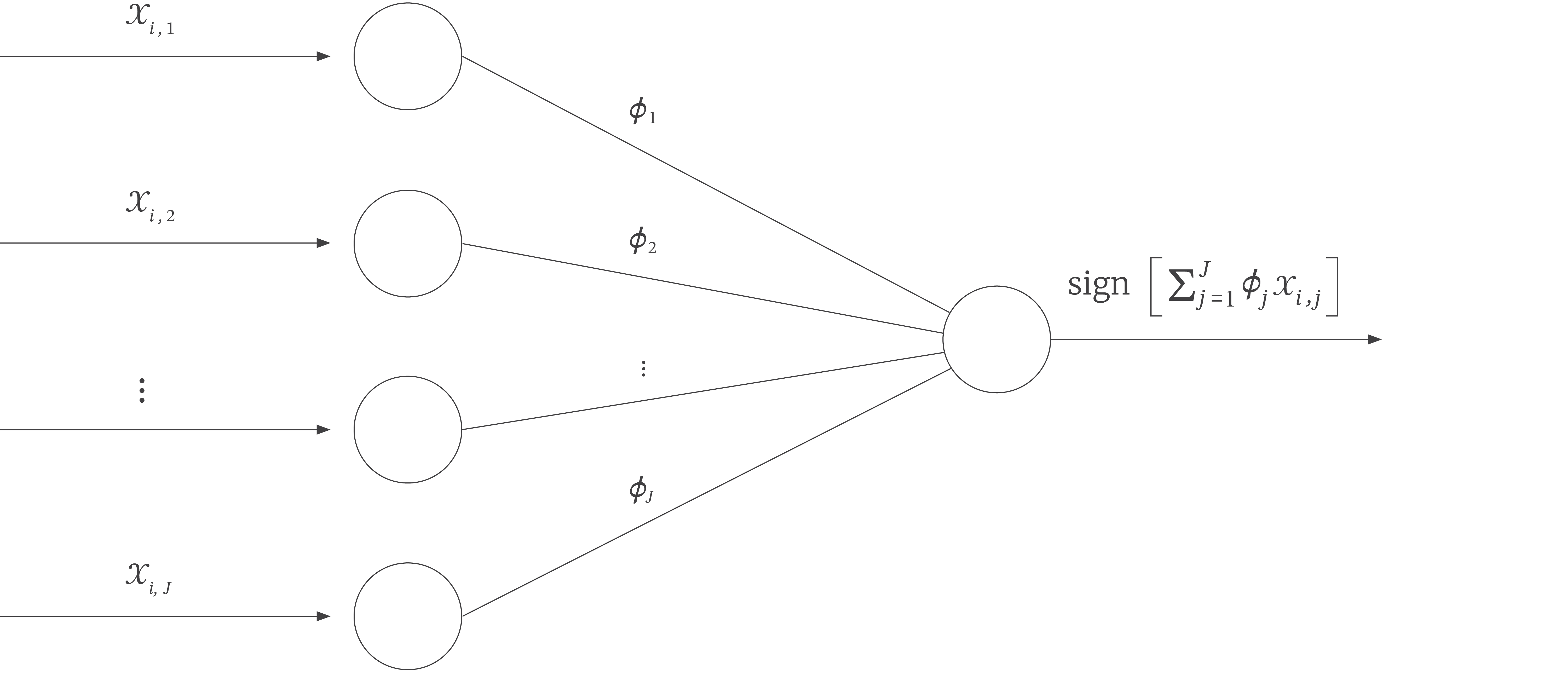
Figure 5. A binary neural network takes a binary data example $\mathbf{x}_{i}$ with $J$ elements $x_{i,j}\in\{-1,1\}$, and multiplies each element with a learned binary parameter $\phi_{j}\in\{-1,1\}$ and sums the results. The output is also binary and is determined by the sign of this sum.
\begin{equation}\label{eq:one_layer} y = \mbox{sign}\left[\sum_{j=1}^{J}\phi_{j}x_{j}\right] \tag{13}\end{equation}
where the unknown model parameters $\phi_{j}$ are also binary and the function $\mbox{sign}[\bullet]$ returns -1 or 1 (figure 5) based on the sign of the summed terms.
Given a training set of $I$ data/label pairs $\{\mathbf{x}_{i},y_{i}\}$, our goal is to choose the model parameters $\phi_{j}$. We’ll force all of the training examples to be classified correctly and so each training example/label pair can be considered a hard constraint on the parameters.
To encode these constraints, we create new variables $z_{i,j}$ that indicate whether the product $\phi_{j}x_{i,j}$ is positive. This happens when either both elements are positive or both are negative, so we can use the $\mbox{Same}[\phi_{j},x_{i,j}]$ construction. Note that for the rest of this discussion we’ll revert to the convention that $x_{i,j}, y_{j}\in\{$$\text{false}$,$\text{true}$$\}$.
The predicted label is the sum of the elements $z_{i,j}$ and will be positive when more than half of the product terms $z_{i,\bullet}$ evaluate to $\text{true}$. Likewise it will be negative if less than half are $\text{true}$. Hence, for the network to predict the correct output label $y_{i}$ we require
\begin{equation}\left(y_{i} \land \mbox{AtLeastK}[\mathbf{z}_{i}]\right)\lor \left(\overline{y}_{i} \land \lnot\mbox{AtLeastK}[\mathbf{z}_{i}]\right) \tag{14}\end{equation}
where $K=J/2$ and the vector $\mathbf{z}_{i}$ contains the product terms $z_{i,\bullet}$.
We have one such constraint for each training example and we logically $\text{AND}$ these together. When we run the SAT solver we are asking whether it is possible to find a set of parameters $\boldsymbol\phi$ for which all of these constraints are met.
It is easy to extend this example to multi-layer networks and to allow a certain amount of training error and we leave these extensions as exercises for the reader.
Fitting decision trees
A binary decision tree also classifies data $\mathbf{x}_{i}$ into binary labels $y_{i}\in\{0,1\}$. Each data example $\mathbf{x}_{i}$ starts at the root. It then passes to either the left or right branch of the tree by testing one of its elements $x_{i,j}$. We’ll consider binary data $x_{i,j}\in\{$$\text{false}$, $\text{true}$$\}$ and adopt the convention that the data example passes left if $x_{i,j}$ is $\text{false}$ and right if $x_{i,j}$ is $\text{true}$. This procedure continues, testing a different value of $x_{i,j}$ at each node in the tree until we reach a leaf node at which a binary output label is assigned.
Learning the binary decision tree can also be framed as a satisfiability problem. From a training perspective, we would like to select the tree structure so that the training examples $\mathbf{x}_{i}$ that reach each leaf node have labels $y_{i}$ that are all $\text{true}$ or all $\text{false}$ and hence the training classification performance is 100%.
We’ll develop a simplified version of the approach of Narodytska et al. (2018). Incredibly, we can learn both the structure of the tree and which features to branch on simultaneously. When we run the SAT solver for a given number $N$ of tree nodes, it will search over the space of all tree structures and branching features and return $\text{SAT}$ if it is possible to classify all the training examples correctly and provide a concrete example in which this is possible. By changing the number of tree nodes, we can find the point at which this problem turns from $\text{SAT}$ to $\text{UNSAT}$ and hence find the smallest possible tree that classifies the training data correctly.
We’ll describe the SAT construction in two parts. First we’ll describe how to encode the structure of the tree as a set of logical relations and then we’ll discuss how to choose branching features that classify the data correctly.
Tree structure: We create $N$ binary variables $v_{n}$ that indicate if each of the $N$ nodes is a leaf. Similarly we create $N^{2}$ binary variables $l_{m,n}$ indicating if node $n$ is the left child of node $m$ and $N^{2}$ binary variables $r_{m,n}$ indicating if node $m$ is the right child of node $n$. Then we build Boolean expressions to enforce the following constraints:
- Each non-leaf node must branch on exactly one feature.
- The left and right ancestor variables at the root are all $text{false}$.
- The left ancestor variables $a^{l}_{bullet, n}$ at a node $n$ are the same as the parent’s, but the index associated with the parents branching variable is also $text{true}$ if we branched left to get here.
- The right ancestor variables $a^{r}_{bullet, n}$ at a node $n$ are the same as the parent’s, but the index associated with the parents branching variable is also $text{true}$ if we branched right to get here.
- You can’t branch on a variable twice in any one path to a leaf.
- A data example reaches a leaf node if the left and right ancestors match its pattern of $text{true}$ and $text{false}$ elements as described above.
- All data that reach a given leaf node must have the same class.
Any set of variables $v_{n}$, $l_{m,n}$, $r_{m,n}$ that obey these constraints form a valid tree, and we can find such a configuration with a SAT solver. Two such trees are illustrated in figure 6.
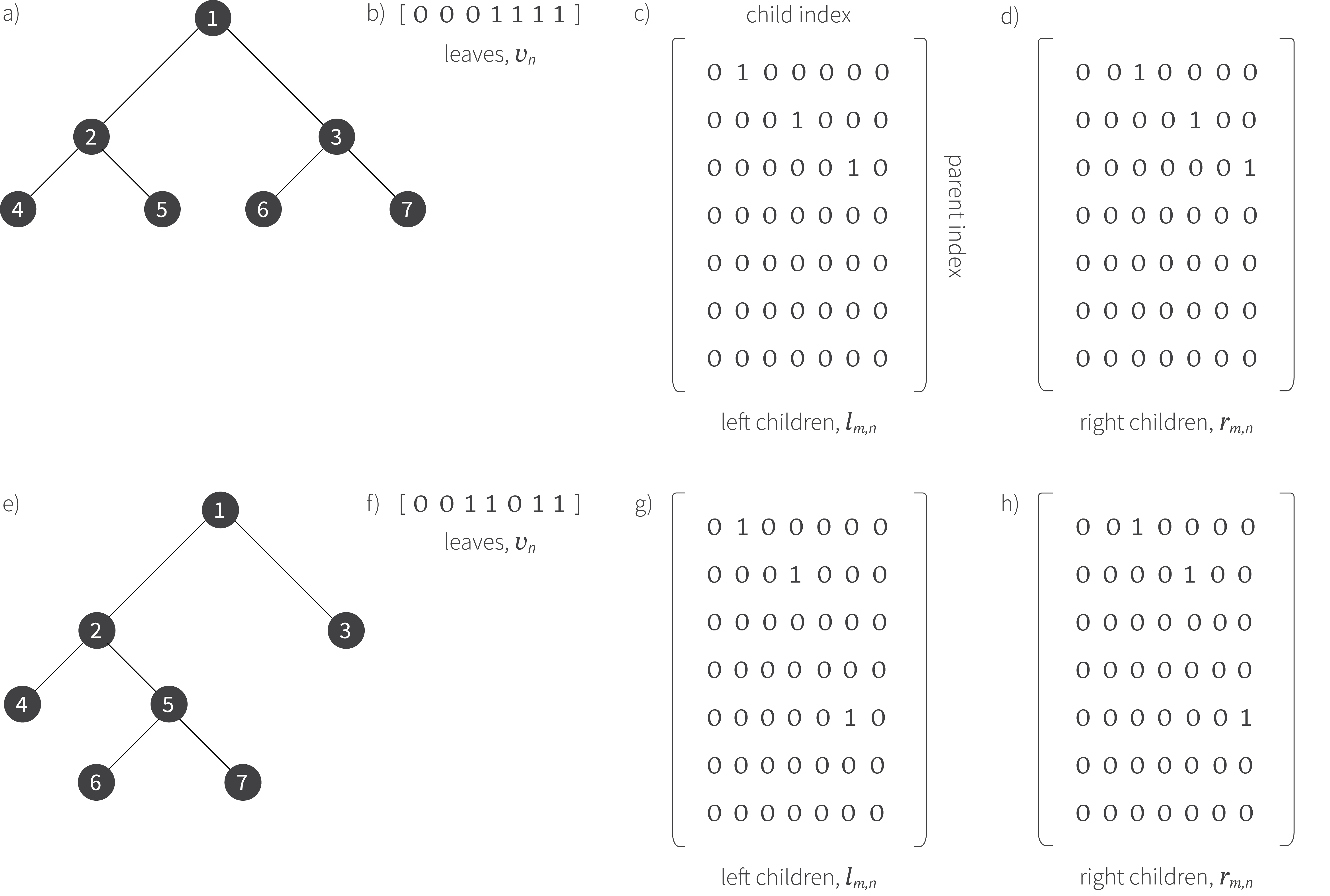
Figure 6. Tree encoding with binary variables. a) Tree with 7 nodes. b) The parameters $v_{n}$ indicate whether the corresponding node is a leaf. So, $v_{2}$ is $\text{false}$ because it is not a leaf, but $v_{6}$ is $\text{true}$ because it is a leaf. c) The parameters $l_{m,n}$ indicate whether node $n$ is a left child of node $m$. So, $l_{2,4}$ is $\text{true}$ because node $4$ is a left child of node $2$. d) Similarly, the parameters $r_{m,n}$ indicate whether node $n$ is a right child of node $m$. e-h) A second tree encoded using the same method.
Classification: The second part of the construction ensures that the data examples $\mathbf{x}_{i}$ are classified correctly (figure 7). We introduce variables $f_{n,j}$ that indicate that node $n$ branches on feature $x_j$. We’ll adopt the convention that when the branching variable $x_{j}$ is $\text{false}$ we will always branch left and when it is $\text{true}$ we will always branch right. In addition, we introduce variables $\hat{y}_{n}$ that will indicate if each leaf node classifies the data as $\text{true}$ or $\text{false}$ (their values will be arbitrary for non-leaf nodes).
We’ll also create several book-keeping variables that are needed to set this up as a SAT problem, but are not required to run the model once trained. We introduce ancestor variables $a^{l}_{nj}$ at each node $n$ which are $\text{true}$ if we branched left on feature $j$ at node $n$ or at any of its ancestors and similarly $a^{r}_{nj}$ if we branched right on feature $j$ at this node or any of its ancestors. Finally, we introduce variables $e_{i,n}$ that indicate that training example $\mathbf{x}_{i}$ reached leaf node $n$. Notice that this happens when $x_{ij}$ is $\text{false}$ everywhere $a^{l}_{nj}$ is $\text{true}$ (i.e., we branched left somewhere above on these left ancestor features) and $x_{ij}$ is $\text{true}$ everywhere $a^{r}_{nj}$ is $\text{true}$ (i.e., we branched right somewhere above on these right ancestor features).
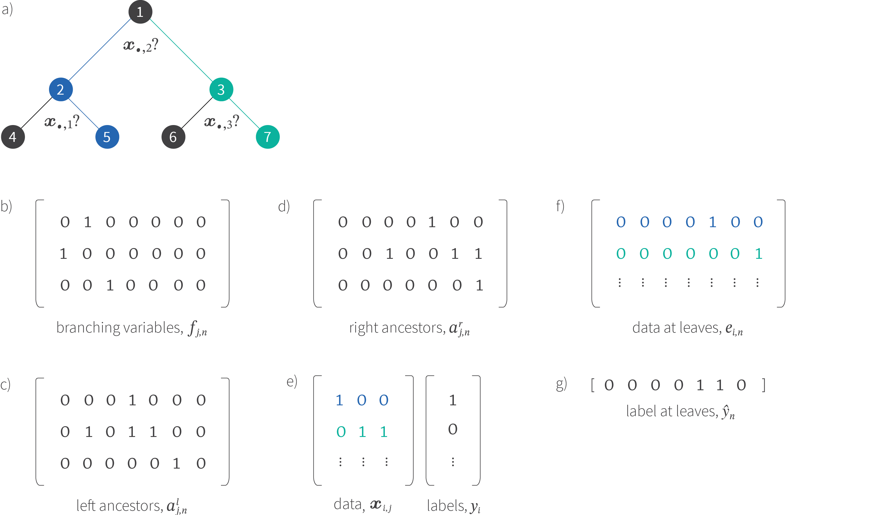
Figure 7. Binary decision tree construction. a) Tree with branching variables. b) The branching index $j$ at each node $n$ is encoded by the variables $f_{j,n}$, so we can see that node 1 branches on element 2 and node 3 branches on element 3. c) The book keeping variables $a^{l}_{j,n}$ indicate if node $n$ or its ancestors branched left on index $j$ . For example, node 4 ($4^{th}$ column) contains two $\text{true}$ values corresponding to the fact that we branched left on variable 2 (at node 1) and variable 1 (at node 2) to arrive here. d) Similarly the right ancestor variables $a^{l}_{j,n}$ keep track of the where we branched right to arrive here. e) The training data consists of $J=3$ dimensional binary examples $x_{i,j}$ (in the rows of the matrix) and each is associated with a binary label $y_{i}$. The first data example is coloured blue and passes through the blue path on the tree. It takes the left path at node 1 which branches on the second dimension because its second element is $\text{false}$. Similarly it branches right at node 2 because its first element is $\text{true}$ . The path of the second variable is similarly indicated in green. f) The variables $e_{i,n}$ are $\text{true}$ if data example $i$ arrives at leaf node $n$. This will be the case if data is $\text{false}$ everywhere the left ancestors $a^{l}_{\bullet,n}$ are $\text{true}$ and the data is $\text{true}$ everywhere the right ancestors $a^{r}_{\bullet,n}$ are $\text{true}$. g) We enforce the constraint that all the data examples that arrive at any leaf must have the same label $\hat{y}_{n}$.
Using these variables, we build Boolean expressions to enforce the following constraints:
- Each non-leaf node must branch on exactly one feature.
- The left and right ancestor variables at the root are all $text{false}$.
- The left ancestor variables $a^{l}_{bullet, n}$ at a node $n$ are the same as the parent’s, but the index associated with the parents branching variable is also $text{true}$ if we branched left to get here.
- The right ancestor variables $a^{r}_{bullet, n}$ at a node $n$ are the same as the parent’s, but the index associated with the parents branching variable is also $text{true}$ if we branched right to get here.
- You can’t branch on a variable twice in any one path to a leaf.
- A data example reaches a leaf node if the left and right ancestors match its pattern of $text{true}$ and $text{false}$ elements as described above.
- All data that reach a given leaf node must have the same class.
Collectively, these constraints mean that all of the data must be correctly classified. When we logically $\text{AND}$ all of these constraints together, and find a solution that is $\text{SAT}$ we retrieve a tree that classifies the data 100% correctly. By reducing the number of nodes until the point that the problem becomes $\text{UNSAT}$, we can find the most efficient tree that partitions the training data exactly.
Conclusion
This concludes part I of this tutorial on SAT solvers. We’ve introduced the SAT problem, shown how to convert it to conjunctive normal form and presented some standard SAT constructions. Finally, we’ve described several different applications which we hope will inspire you to see SAT as a viable approach to your own problems.
In the next part of this tutorial, we’ll delve into how SAT solvers actually work. In the final part, we’ll elucidate the connections between SAT solving and factor graphs. For those readers who still harbor reservations about the applicability of a method based purely on Boolean variables, we’ll also consider (i) how to convert non-Boolean variables to binary form and (ii) methods to work with them directly using SMT solvers.
Further reading
If you want to try working with SAT algorithms, then this tutorial will help you get started. For an extremely comprehensive list of applications of satisfiability, consult SAT/SMT by example. This may give you more inspiration for how to re-frame your problems in terms of satisfiability.
Work with Us!
Impressed by the work of the team? RBC Borealis is looking to hire for various roles across different teams. Visit our career page now and discover opportunities to join similar impactful projects!
Careers at RBC Borealis