Tutorial #13: Differential privacy II: machine learning and data generation

In part I of this tutorial we discussed what it means for data analysis to be “private” with respect to a dataset and argued that perfect privacy is not possible. Instead, privacy assurances must be balanced with the utility of the analysis; this led to the notion of differential privacy (DP) and we discussed differentially private mechanisms for some basic calculations.

In part II of the tutorial, we present recent methods for making machine learning differentially private. We will also discuss differentially private methods for generative modelling which provide an enticing solution to a seemingly intractable problem: how can we release data for general use while still protecting privacy?

Machine learning with differential privacy

Most machine learning algorithms optimize an objective function representing how well the training data has been learned. This optimization is typically performed using a variant of stochastic gradient descent (SGD). The near universality of SGD makes it a natural starting point for differentially private machine learning. Moreover, the inherent randomness of SGD suggests a natural affinity with differential privacy.

DP-SGD

DP-SGD (Algorithm 1) is similar to traditional stochastic gradient descent. We first randomly initialize the parameters, then proceed by randomly selecting a batch of data points, computing their gradients, and using those gradients to update the parameters. The key differences are the lines highlighted in blue in which the gradient norms are clipped, and those highlighted in red where Gaussian noise is added.

Algorithm 1: Differentially private stochastic gradient descent

Input: Training data $\mathcal{D} = \{\mathbf{x}_1,\dots, \mathbf{x}_I\}$; Loss function $\mathcal{L}[\boldsymbol\theta] = \frac{1}{I}\sum_i\mathcal{L}[\boldsymbol\theta,\mathbf{x}_i]$; Parameters: learning rate $\eta_t$, noise scale $\sigma$, batch size $B$, gradient norm bound $C$Initialize $\boldsymbol\theta_0$ randomly
for $t=1,\dots,T$ do

Randomly sample a batch $\mathcal{D}_t \subset \mathcal{D}$
Compute the gradient $\mathbf{g}_t[\mathbf{x}_i] = \nabla_{\theta} \mathcal{L}[\boldsymbol\theta_{t-1},\mathbf{x}_i]$ for each $\mathbf{x}_i \in \mathcal{D}_t$

Clip the magnitude of each gradient
\begin{equation}
\mathbf{g}_t[\mathbf{x}_i] \leftarrow \frac{\mathbf{g}_t[\mathbf{x}_i]}{\max\left[1,\Vert \mathbf{g}_t(\mathbf{x}_i) \Vert/C\right]}
\end{equation}
Add noise $\boldsymbol\xi_{i,t}\sim \mbox{Norm}_{\boldsymbol\xi_{i,t}}[\mathbf{0},\sigma^{2}C^{2}\mathbf{I}]$
\begin{equation}
\mathbf{g}_t[\mathbf{x}_i] \leftarrow \mathbf{g}_t[\mathbf{x}_{i}] + \boldsymbol\xi_{i,t} 
\end{equation}
Average the (clipped, noisy) gradients
\begin{equation}
\bar{\mathbf{g}}_t = \frac{1}{B} \sum_{x_i\in{D}_{t}} \mathbf{g}_t[\mathbf{x}_i]
\end{equation}
Take a step in the descent direction
\begin{equation}
\boldsymbol\theta_t \leftarrow \boldsymbol\theta_{t-1} – \eta_t\bar{\mathbf{g}}_t
\end{equation}

end
Output: Final parameters $\boldsymbol\theta_T$

In part I, we saw that DP mechanisms are sensitive to worst case scenarios and a single data point that produces an arbitrarily large gradient could violate privacy by having an out-sized influence on the final model. Hence, the magnitude of the gradient contribution from each data point is limited to be no more than $C$. Gaussian noise is then added to each gradient. In part I of this tutorial, we saw that for a fixed level of differential privacy, there is a connection between the amount of noise we must add and the amount of clipping. A larger value of $C$ does less clipping, but requires more noise to retain the same degree of privacy and this is made explicit in the algorithm.

The process of clipping, adding Gaussian noise, and averaging together the gradients in the mini-batch is differentially private. As we train, we combine the gradients from different mini-batches, and this too is differentially private due to the composition properties of differential privacy. However, this can significantly over-estimate how much privacy is lost.

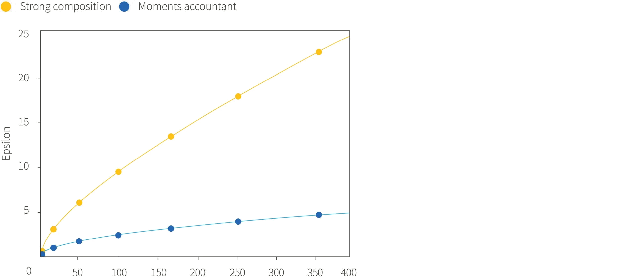
Consequently, Abadi et al. (2016) developed a method to keep better track of privacy loss, which was termed the moments accountant. While the details are beyond the scope of this tutorial, the empirical results are shown in figure 1. For a given noise level and number of training steps, the moments accountant results in a much smaller value of $\epsilon$ and hence a much better guarantee on privacy. The learned model is identical whichever way we track the privacy loss, but for a given privacy budget, the moments accountant allows DP-SGD to be run for many more iterations.

DP-SGD performance

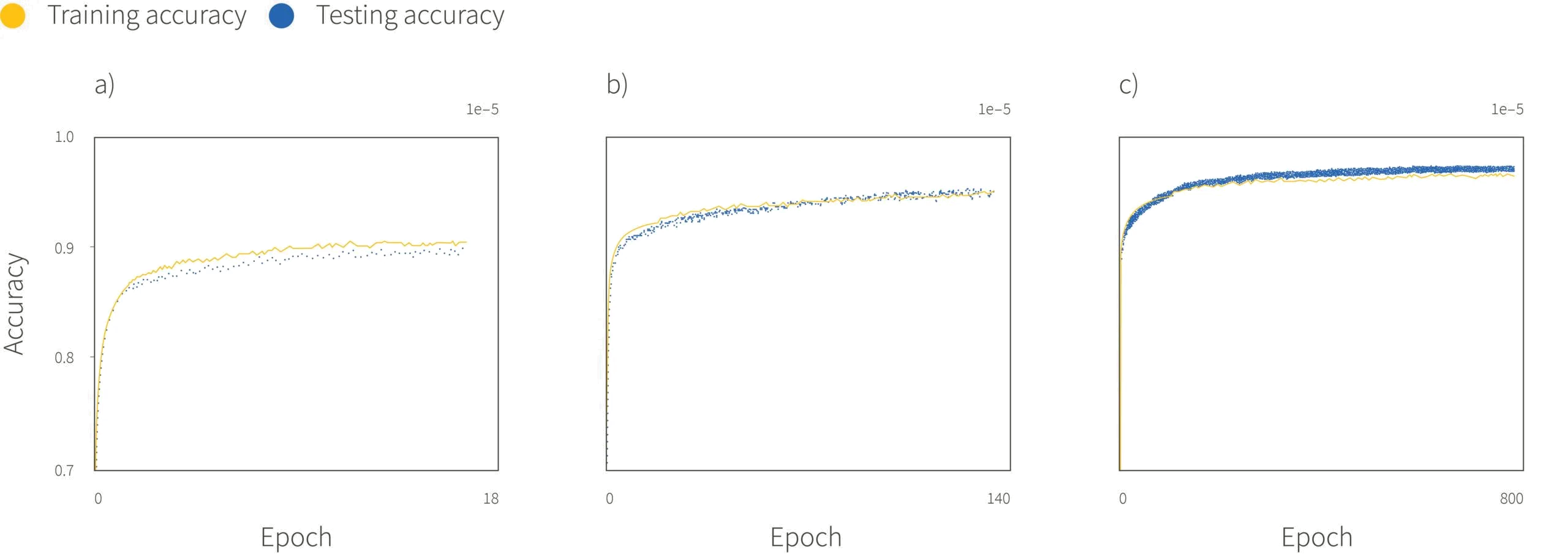
We have established how to learn a machine learning model using a differentially private mechanism. However, we have not yet addressed the question of how this impacts model performance. Abadi et al. (2016) found that smaller privacy budgets tended to produce lower accuracy on the test set (figure 2). However, an interesting upside was that differentially private SGD improved generalization performance; the gap between training and testing accuracy tended to be smaller, particularly for smaller privacy budgets. Although this may initially appear counter-intuitive, it is perhaps not entirely surprising given that there are strong theoretical parallels between generalization and differential privacy and it is known that adding noise during training can improve generalization.

PATE

In the previous section, we described a differentially private version of stochastic gradient descent. While stochastic gradient descent is the most popular ML training algorithm, there are many other useful techniques, including boosting, decision trees, nearest neighbours, and others. Papernot et al. (2017) introduced a framework for differentially private learning known as Private Aggregation of Teacher Ensembles or PATE that allows any model to be used during training.

PATE works by making the predictions of the machine learning model differentially private instead of making the model itself differentially private. Consider a machine learning model $\mbox{f}[\cdot;\boldsymbol\theta]$ with parameters $\boldsymbol\theta$. The DP-SGD method described above trains the model $\mbox{f}[\cdot;\boldsymbol\theta]$ such that the parameters $\boldsymbol\theta$ are private and by extension any predictions that are derived from them. Alternatively, we could train the model using a standard algorithm. We cannot release the parameters $\boldsymbol\theta$ but we can release the predictions of the model if we add noise using a randomized response mechanism. However, every time we make a prediction, we spend privacy and so we could only ever make a finite number of predictions for a fixed privacy budget.

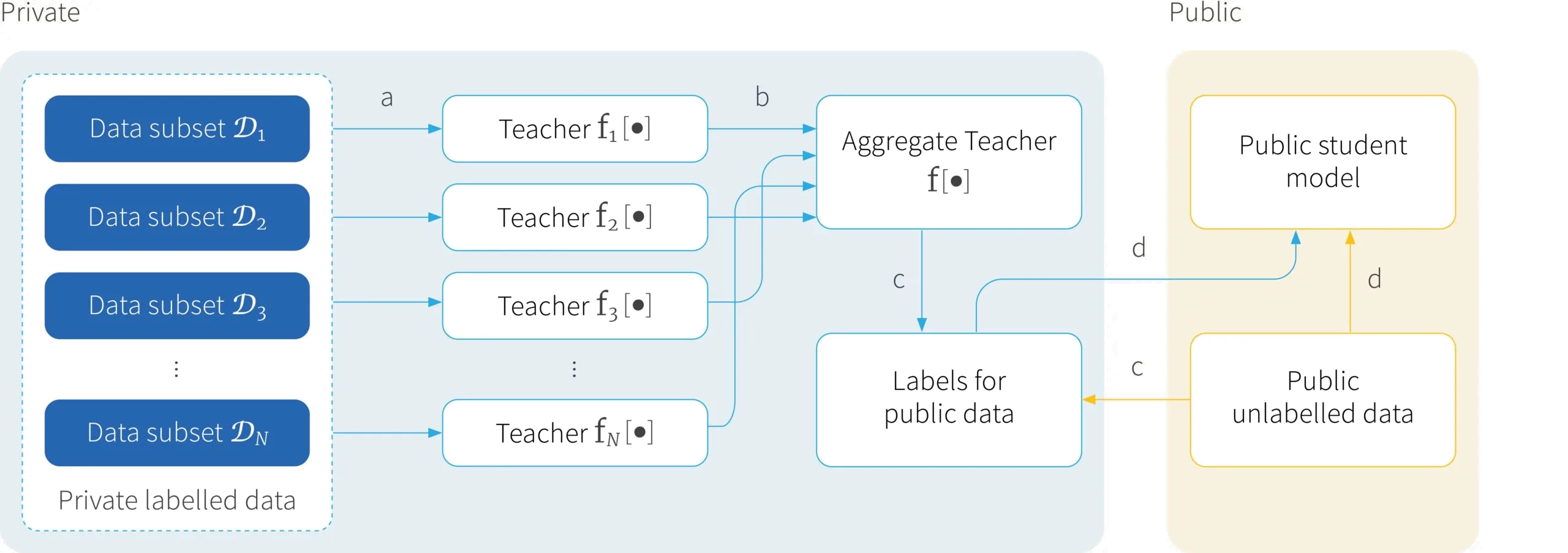
PATE combines the advantages of both of these approaches. It allows any model to be used to make the predictions, and allows that model to be queried an arbitrary number of times without leaking privacy. However, to accomplish this, it assumes that we have a additional trove of unlabelled public (non-sensitive) data. The overall idea is to use the private data to label this public data such that the labels are differentially private and then use this new labelled data to train any new model we want (figure 3).

In more detail, PATE divides the sensitive data into $N$ disjoint subsets $\mathcal{D}_{1}\ldots \mathcal{D}_{N}$, each of which is used to train an independent machine learning model $\mbox{f}_{n}[\mathbf{x}]$ known as a teacher. Then, these teachers are combined to create an aggregate teacher using a noisy voting model:

\begin{equation}\mbox{f}[\mathbf{x}] = \underset{j}{\operatorname{argmax}} \left[ \sum_{n}[f_{n}[\mathbf{x}]=j] + \xi \right]. \tag{1}\end{equation}

Here, we count how many of the $n$ classifiers give answer $j$ and add noise $\xi\sim\mbox{Lap}_{\xi}[\epsilon^{-1}]$ from a Laplacian distribution with parameter $b=\epsilon^{-1}$ to get a vote for class $j$. Then we choose the class with the largest vote.

This differentially private model can only make a finite number of predictions before expending its privacy budget. PATE uses this finite number of predictions to label the public (non-sensitive data). This creates a differentially private dataset from which any type of model can be trained. By the post-processing property of differential privacy, this student model will also be differentially private.

PATE results

Papernot et al. (2017) applied PATE on MNIST and SVHN and in a followup paper introduced new aggregation techniques, tighter privacy bounds, and applied the technique on more datasets. They showed that the models produced from the PATE framework either significantly outperformed other differentially private learning approaches in terms of accuracy or privacy budget required. In many cases, PATE was better on both fronts, producing higher test set accuracy with lower privacy budgets.

PATE analysis

The PATE framework is straightforward but it is not obvious why it needs multiple teachers. Couldn’t we set $N=1$, train a single teacher on the entire dataset, and use a different privacy mechanism to label the data? The answer is yes, but in fact a significant amount of privacy is gained through splitting the dataset and aggregating the outputs of the teachers.

To understand why, recall that differential privacy is based on what happens when we change a single element in our dataset. With data splitting and teacher aggregation, that single element change can only affect a single teacher and because of the voting mechanism, this is less likely to change the result; a change in a single element can only change the result when the voting is close.

This insight is exploited in the followup paper to derive a data dependent bound on the privacy budget spent when labelling the public data. Labelling inputs which produce near ties expends significantly more privacy than labelling inputs which have clear consensus among the teachers. This argues for more teachers. Near ties in the voting are less likely when there are more teachers and so less noise needs to be added during aggregation. This idea can be used to reduce the privacy budget used by allowing the aggregate teacher to refuse to label inputs where there isn’t sufficient consensus.

Of course, there is a limit on the benefit of adding more teachers. As the number of teachers increase, the number of data points used to train each teacher decreases and so does its accuracy; while having more teachers may reduce the amount of noise added to the labels for the student it will, eventually, decrease the accuracy of those labels.

Differentially private data generation

In the previous section we introduced methods for building machine learning models that make predictions that are differentially private. We now turn to methods for generating data that are differentially private.

The Netflix Prize competition demonstrated that there is significant power in releasing data for public machine learning challenges. Netflix’s own algorithm was beaten within days in 2006 and the top prize was claimed in 2009. However, Naryan and Shmatikov (2006) showed that it was possible to identify individual Netflix users using a linkage attack in which the dataset was matched with film ratings from the Internet Movie Database

In fact, there are many situations where companies may wish to share data with each other without compromising privacy. For example, pooling medical records between hospitals might be particularly useful when the data pertains to rare diseases. In such situations, organizations wish to protect the privacy of the data without preventing their researchers from doing their jobs. The answer to this conundrum is not to release the data at all. Instead we can release synthetic data which looks and acts like the real data, but which has been generated in a differentially private manner.

A generative model takes a dataset and learns how to synthesize realistic new examples. This area of machine learning has seen enormous success in recent years. It is now possible to generate compelling but purely synthetic images of people, cats, horses, artwork and even chemicals.

Generative adversarial networks

A successful type of generative model is the Generative Adversarial Network (GAN). This consists of two networks: a generator, $G[\mathbf{z};\boldsymbol\theta)]$ and a discriminator $D[\mathbf{x};\boldsymbol\phi]$. The generator is a network with parameters $\boldsymbol\theta$ that takes a sample of random noise $\mathbf{z}$, and transforms this into a data point $\mathbf{x}$. The discriminator is a second network with parameters $\boldsymbol\phi$ that takes a data point $\mathbf{x}$ and seeks to classify that data point as being either real data or fake (i.e., created by the generator).

Training a GAN can be thought of as a two-player game in which the discriminator tries to identify which data points are fake, and the generator tries to generate data points which fool the discriminator. The players take turns updating their parameters by taking steps of stochastic gradient descent based on the current state of the other player. The generator takes a few steps of SGD trying to minimize

\begin{equation}\min_{\boldsymbol\theta} \left[-\mathbb{E}_{\mathbf{z}}[\log D[G[\mathbf{z};\boldsymbol\theta];\boldsymbol\phi]]\right],\tag{2} \end{equation}

followed by the discriminator taking steps of SGD trying to maximize

\begin{equation}\max_{\boldsymbol\phi} \left[\mathbb{E}_{x}[\log D[\mathbf{x};\boldsymbol\phi]] – \mathbb{E}_{\mathbf{z}}[\log D[G[\mathbf{z};\boldsymbol\theta];\boldsymbol\phi]]\right]. \label{eq:GAN_D}\tag{3} \end{equation}

Here, the expectations $\mathbb{E}_\mathbf{x}$ and $\mathbb{E}_\mathbf{z}$ are approximated by taking samples from the training data and noise distributions respectively. Once this game has converged, samples can be generated by sampling a noise vector $\mathbf{z}$ and feeding it through the generator $G[\mathbf{z};\boldsymbol\theta]$.

DP-GAN

In the previous section we saw that GAN training is based on stochastic gradient descent. The DP-GAN applies the differentially private SGD method of Abadi et al. to learning a GAN; it applies gradient clipping and adds Gaussian noise as described previously and uses the moments accountant to track the privacy budget.

Note that the real data (whose privacy we want to protect) is only present in the discriminator where real samples are compared to the generated ones. Consequently, we update the discriminator with DP-SGD. The generator is updated only based on the discriminator and hence can be updated using standard SGD. This will be differentially private based on the post-processing theorem and any generated samples, or even the entire generator itself, can be released without further compromising the privacy of the data.

Unfortunately, the performance of DP-GAN is relatively poor in practice. Large privacy budgets were required to produce plausible results even on relatively simple datasets like MNIST and generated images using plausible privacy budgets were of low quality. Subsequent work has improved matters. Frigerio et al. (2019) developed better gradient clipping strategies while applying DP-GAN to a broader range of data domains. Torkzadehmahani et al. (2019) introduced an improved privacy accounting method based on Renyi differential privacy and used their framework for training conditional GANs.

PATE-GAN

In the previous section, we argued that using DP-SGD to train GANs is possible but does not produce good results for reasonable privacy budgets. PATE-GAN is an alternative apporach that leverages the PATE framework to train differentially private GANs.

As we saw above, it is only the discriminator which needs to be differentially private; the generator is updated based on the discriminator and so inherits the differential privacy due to the post-processing property. Since the discriminator is just a classifier which labels its input as either “real” or “fake”, we could replace this with the student model from a PATE-trained classifier.

Recall that PATE requires a non-sensitive, unlabelled dataset which is used to query the differentially private aggregated teacher model to produce labels. The dataset and its labels are then used to train the student classifier. In PATE-GAN, we use the generator in place of this unlabelled dataset. The samples from the generator are used to query the teachers and the resulting labels are used to train the student.

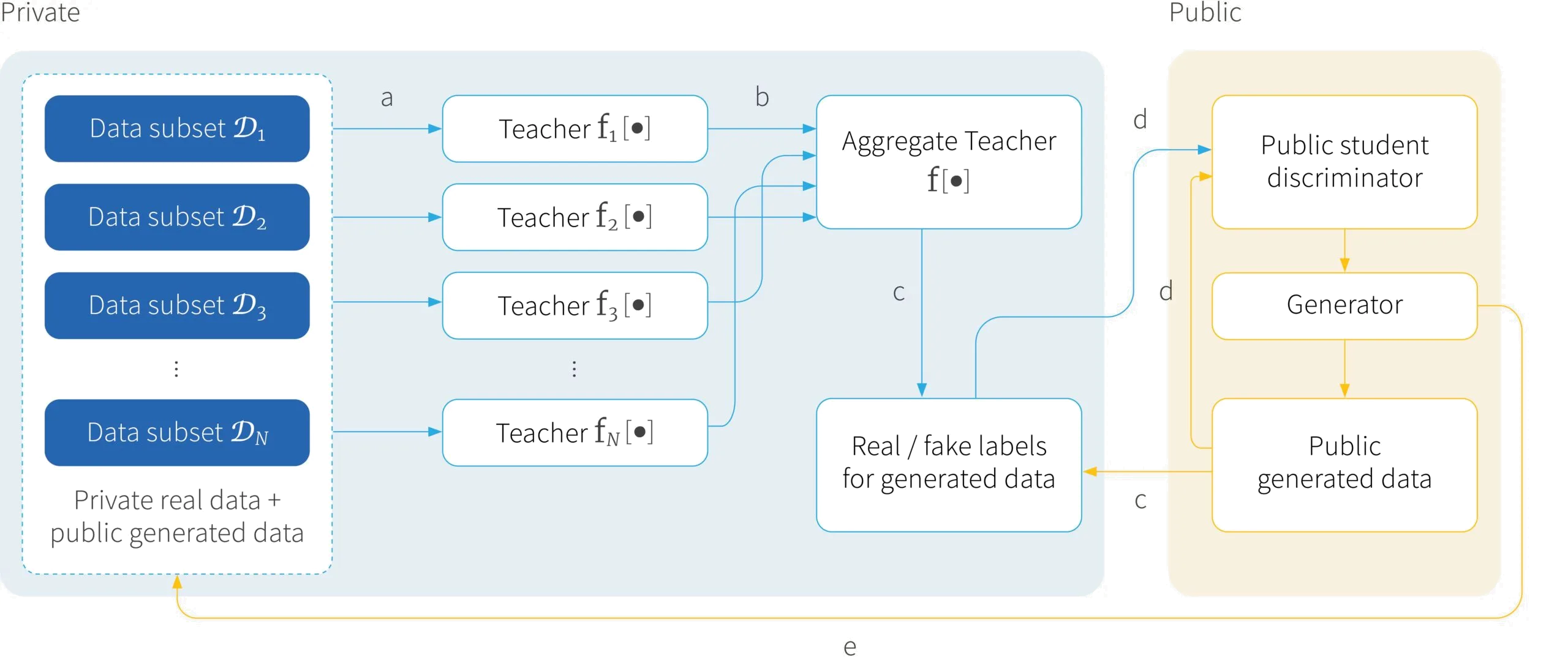
In a GAN, the generator and discriminator must be trained in concert. However, training the discriminator is no longer as simple as a few SGD steps. Instead, PATE-GAN alternates between (i) using the generator to produce samples which are then combined with real data to update the teachers, (ii) using the generator to produce samples which are then used to query the (updated) teachers to produce labelled samples which are used to update the student model, and then finally (iii) using the student model to update the generator (figure 4).

PATE-GAN evaluation

The performance of PATE-GAN was not primarily evaluated in terms of the sample quality. Instead, the authors measure performance for the scenario where a real dataset is replaced with a synthetic one. To this end, the generator was used to produce a training set, which was used to train a new model, and finally tested against real data.

Using this criterion, performance with PATE-GAN was significantly better than with DP-GAN given the same privacy budget, although it was worse than training directly on the real data for some datasets. However, performance was only slightly worse than using the same method with a non-differentially private GAN. This implies that the performance gap is not specific to differential privacy, but rather a limitation of current generative models.

Private data generation is known to be theoretically hard in the worst case. However, the properties of non-convex optimization suggest that theoretically deep learning should be nearly impossible and yet we do it in practice every day. Likewise, it seems that private data generation may also be practically feasible. There is much research to be done in this area. There are a plethora of other generative models beyond GANs (VAEs, normalizing flows, implicit likelihood models, etc.) which are ripe for DP analysis and many other open questions. Nonetheless, algorithms like PATE-GAN already provide practically useful differentially private data generation which may be sufficient in some cases.  One useful resource in this area is our open-source toolbox that implements PATE-GAN and several other methods for private data generation.

Conclusion

Part I of this tutorial introduced differential privacy generally and showed basic examples of differentially private data analysis. In part II we have discussed state-of-the-art techniques for applying modern machine learning in a differentially private manner. Whether the goal is to learn a single, private machine learning model from sensitive data, or to enable the release of new datasets, there are differentially private options. Machine learning with sensitive data does not have to come at the expense of privacy.