
Part I of this series of articles discussed ordinary differential equations (ODEs) and stochastic differential equations (SDEs) and outlined their applications to machine learning. Part II introduced ordinary differential equations. We saw that the solution to an ODE is a family of functions and that the relationship between the members of the family depends on properties such as time invariance, linearity, linear homogeneity, and Euler homogeneity. Additional boundary constraints identify a particular solution from this family.
This article (part III) describes methods for solving ordinary differential equations. We restrict our discussion to first-order ODEs, which are the type that are most commonly applied to machine learning. These have the form:
\begin{equation}
\frac{d\mathbf{x}}{dt} = \textbf{f}[\mathbf{x},t],
\tag{1}
\end{equation}
where a solution is a vector function $\textbf{x}[t]$ indicating how the vector dependent variable $\textbf{x}\in\mathbb{R}^{D}$ varies over time. Unfortunately, there is no known method to solve an arbitrary first-order ODE in closed form (i.e, to yield a mathematical expression for $\textbf{x}[t]$). However, methods are known for some classes of ODE, and we describe these techniques in this article. For the remaining ODEs to which no solution method is currently available, we apply numerical methods to simulate paths through the ODE. We wil describe these in the subsequent article in this series.
Closed-form solutions (scalar)
We’ll start by considering ODEs where the dependent variable $x\in\mathbb{R}$ is a scalar. This is not typical in machine learning; the dependent variable usually represents the parameters of a model, or the data representation. However, scalar ODEs are straightforward to understand and easy to visualize, and the solution methods often translate to the vector case. Scalar ODEs have the general form:
\begin{equation}
\frac{dx}{dt} = \textrm{f}[x,t].
\tag{2}
\end{equation}
Even in the scalar case, it is not always possible for find a closed-form expression for the family of solutions; neither the individual members of this family, nor the relationship between are necessarily simple.
Validating proposed solutions
Not all equations have known solutions, and even if we do have a proposed solution, it’s correctness may not be obvious by inspection. However, it is easy to check if a proposed solution $\textrm{x}[t]$ is valid. We simply compute its derivative and see if it matches the right-hand side. For example, given the linear ODE:
\begin{equation}\label{eq:ode3_check_eqn}
\frac{dx}{dt} = a x,
\tag{3}
\end{equation}
we can easily verify that the general solution is
\begin{equation}\label{eq:ode3_proposed_solution}
x = C\exp[a t]
\tag{4}
\end{equation}
where $C$ is an arbitrary constant $C$. To do this, we compute the derivative of the proposed solution:
\begin{equation}
\frac{dx}{dt} = \frac{d}{dt} C\exp[a t] = aC \exp[a t] = a\cdot x,
\tag{5}
\end{equation}
which is exactly the right-hand side of the original ODE (equation 3).
Classes of ODEs with solutions
This section lists some of the classes of ODE for which there exist techniques to find closed-form solutions (figure 1). If you need to solve a first-order ODE, the first line of attack is to identify if it falls within one of these classes:
1. Right-hand side is a function of $t$ only:
\begin{equation}
\frac{dx}{dt} = \textrm{f}[t].
\tag{6}
\end{equation}
2. Linear homogeneous:
\begin{equation}
\frac{dx}{dt} = ax.
\tag{7}
\end{equation}
3. Right-hand side is function of $x$ only (time-invariant):
\begin{equation}
\frac{dx}{dt} = \textrm{g}[x].
\tag{8}
\end{equation}
4. Right-hand side is a separable function of $x$ and $t$:
\begin{equation}
\frac{dx}{dt} = \textrm{f}[t]\textrm{g}[x].
\tag{9}
\end{equation}
5. Exact equations:
\begin{equation}
\frac{dx}{dt} = -\left(\frac{\partial \textrm{p}[x,t]}{\partial x}\right)^{-1}\frac{\partial \textrm{p}[x,t]}{\partial t}.
\tag{10}
\end{equation}
6. Linear inhomogeneous:
\begin{equation}
\frac{dx}{dt} = ax + \textrm{f}[t].
\tag{11}
\end{equation}
7. Euler homogeneous:
\begin{equation}
\frac{dx}{dt} = \textrm{h}\left[\frac{x}{t}\right].
\tag{12}
\end{equation}

Figure 1. Classes of ODE with simple closed-form solutions. a) Right-hand side is a function of $t$ only (notice that rows of arrows are all the same as the highlighted red row). b) Linear homogeneous, c) which is a special case of the class of ODEs where the right-hand side is a function of $x$ only (notice that the columns of arrows are all the same as the highlighted red column). d) All three of the previous classes are special cases of separable functions where the right-hand side is a product of a function of $x$ and another function of $t$. e) These separable ODEs are themselves special cases of the broader class of exact ODEs. Certain other classes of ODE such as f) linear inhomogeneous and g) Euler homogeneous can be solved by a change of variable that converts the problem to a separable ODE or one of its special cases.
where $a$ is a scalar factor and $\textrm{f}[t]$, $\textrm{g}[x]$,$\textrm{p}[x,t]$, and $\textrm{h}[x/t]$ are functions of the independent variable, the dependent variable, both variables, and their ratio respectively. The following seven sections contain the derivations for these types of ODE.
Class 1: Right-hand side is a function of t only
Consider an ODE of the form:
\begin{equation}
\frac{dx}{dt} = \textrm{f}[t],
\tag{13}
\end{equation}
where the right-hand side depends on $t$ alone. Two examples are shown in figure 2.
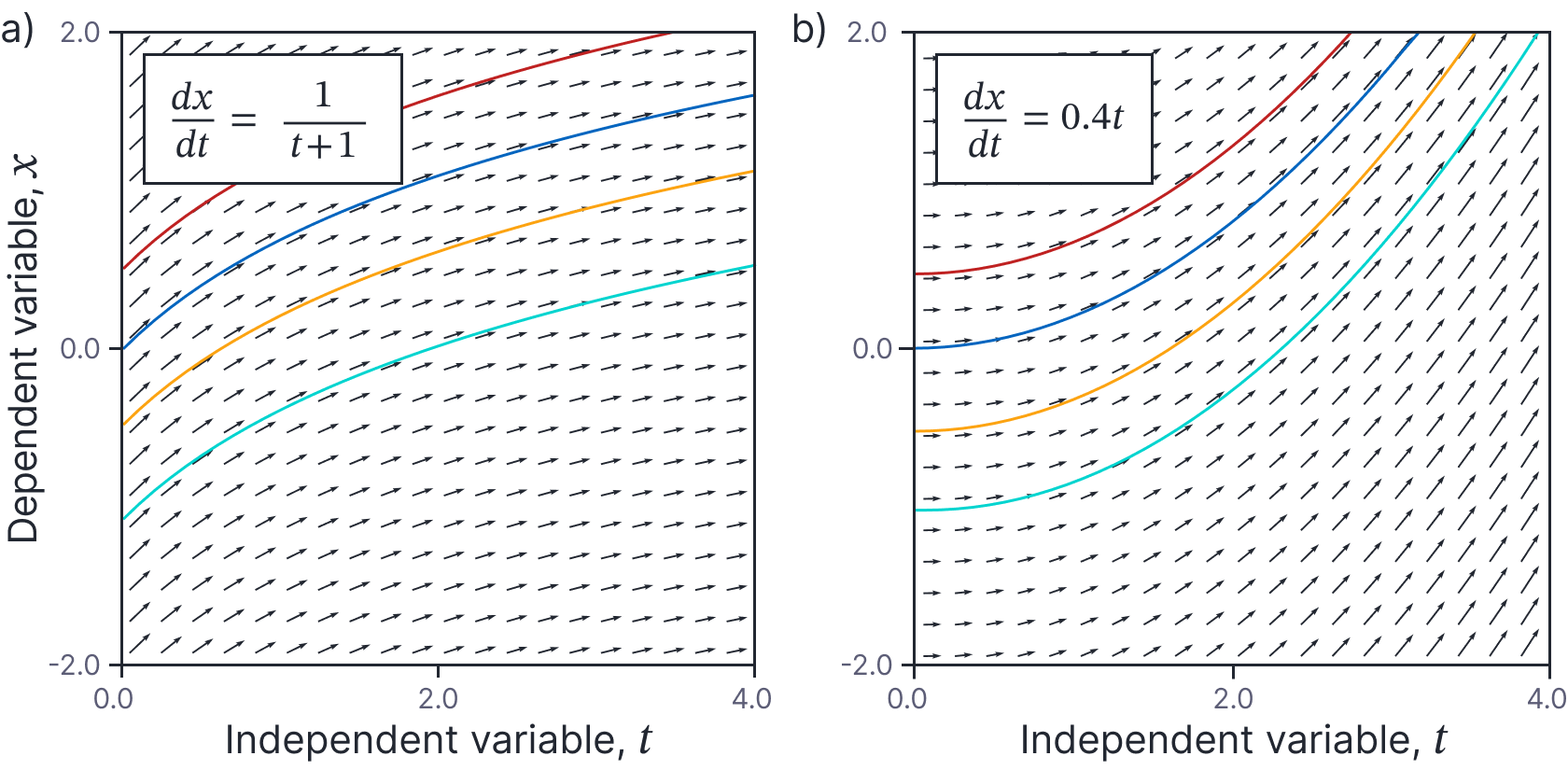
Figure 2. Class 1. right-hand side is a function of $t$ only. a-b) Two examples. Note that in each case, the flow field is the same at each value of the dependent variable $x$ (i.e., the rows of arrows are all identical). The solutions are related by a vertical offset in this plot.
Solution: To solve this equation, we simply integrate the left- and right-hand sides with respect to $t$, which gives:
\begin{equation}
x = C + \int\textrm{f}[t]dt,
\tag{14}
\end{equation}
where $C$ is an arbitrary constant. Here, there is a family of solutions, each of which is related by an additive constant. We term this the general solution.
Example: Consider the ODE:
\begin{equation}
\frac{dx}{dt} = \frac{1}{t+1},
\tag{15}
\end{equation}
with boundary conditions $x=-0.5$ at time $t=0$. This has the general solution:
\begin{eqnarray}
x &=& \int\frac{1}{t+1}dt \nonumber \\
&=& \log[t+1]+ C.
\tag{16}
\end{eqnarray}
When we substitute in the boundary condition we see that:
\begin{eqnarray}
-0.5 = \log[1]+C\quad\quad \implies C = -0.5,
\tag{17}
\end{eqnarray}
which gives the particular solution:
\begin{eqnarray}
x = \log[t+1]-0.5.
\tag{18}
\end{eqnarray}
This is the orange line in figure 2a.
Class 2: Linear homogeneous
The previous family of ODEs had a function of $t$ only on the right-hand side. Now we turn to ODEs where the right-hand side is a function of $x$ alone. We start with the special case where the right-hand side is a multiple $a$ of $x$:
\begin{equation}
\frac{dx}{dt} = a x.
\tag{19}
\end{equation}
This is a linear homogeneous ODE. It is linear because all terms are proportional to $x$ and its derivatives. It is homogeneous because there is no term in $t$ alone. Two examples are depicted in figure 3.

Figure 3. Class 2. Linear homogeneous first-order ODEs where the right-hand side has the form $ax$. a) When $a$ is positive, the solutions correspond to exponential growth. b) When $a$ is negative, the solutions correspond to exponential decay. The solutions can be equivalently thought of as related by either (i) scaling in $x$ or (ii) by shifting in $t$.
Solution: We re-arrange as:
\begin{equation}\label{eq:linear_homog_rearrange}
\frac{1}{x}\frac{dx}{dt} = a,
\tag{20}
\end{equation}
and now we note that the left-hand side is the derivative of $\log[x]$ with respect to $t$:
\begin{equation}
\frac{d\log[x]}{dt}= \frac{d\log[x]}{dx}\frac{dx}{dt} = \frac{1}{x}\frac{dx}{dt},
\tag{21}
\end{equation}
and so integrating both sides of equation 20 with respect to $t$, we get:
\begin{equation}
\log[x] = a\cdot t+A,
\tag{22}
\end{equation}
where $A$ combines the arbitrary integration constant from both sides of the equation. Exponentiating both sides yields:
\begin{equation}
x = \exp\Bigl[a\cdot t+A\Bigr].
\tag{23}
\end{equation}
This is general solution to the equation. Depending on whether $a$ is positive or negative, the solution to the ODE will be either an exponentially increasing or an exponentially decreasing function.
Note that since $A$ is an arbitrary constant, we could equivalently express this general solution in either of the following two forms:
\begin{equation}
x = \exp\Bigl[a\cdot(t+B)\Bigr],
\tag{24}
\end{equation}
where $B=A/a$ is a new arbitrary constant or
\begin{equation}\label{eq:ode3_lin_homog_soln}
x = C\exp\bigl[at\bigr],
\tag{25}
\end{equation}
where $C=\exp[aB]$ is a another new arbitrary constant.
The first of these new formulations emphasizes a property that is true for any first-order ODE where the right-hand side is a function of $x$ alone: if $x[t]$ is a solution, then so is $x[t+B]$. The second emphasizes a property that is true for linear homogeneous first-order ODEs: if $x[t]$ is a solution, then $C x[t]$ is also a solution. In other words, we can equivalently find new solutions by either shifting the current solution with regard to time, or by scaling it in $x$.
Example: Consider the linear homogeneous equation:
\begin{equation}
\frac{dx}{dt} = 0.5 x,
\tag{26}
\end{equation}
with boundary condition $x[0]=-0.2$. Using equation 25 we identify that the general solution is:
\begin{equation}
x = C\exp\bigl[0.5 t\bigr].
\tag{27}
\end{equation}
Substituting the boundary condition $x=-0.2$ at time $t=0$, we can solve to find that $C=-0.2$ and so the particular solution is:
\begin{equation}
x = -0.2 \exp\bigl[0.5 t\bigr].
\tag{28}
\end{equation}
This solution is the orange line in figure 3a.
Class 3: right-hand side is function of x alone:
Consider an ODE where the right-hand side is an arbitrary function $\textrm{g}[x]$ of $x$ alone:
\begin{equation}
\frac{dx}{dt} = \mbox{g}[x].
\tag{29}
\end{equation}
The previously-discussed linear homogeneous case where the right-hand side is $\mbox{g}[x]=ax$ is a special case of this class. Two examples are shown in figure 4.
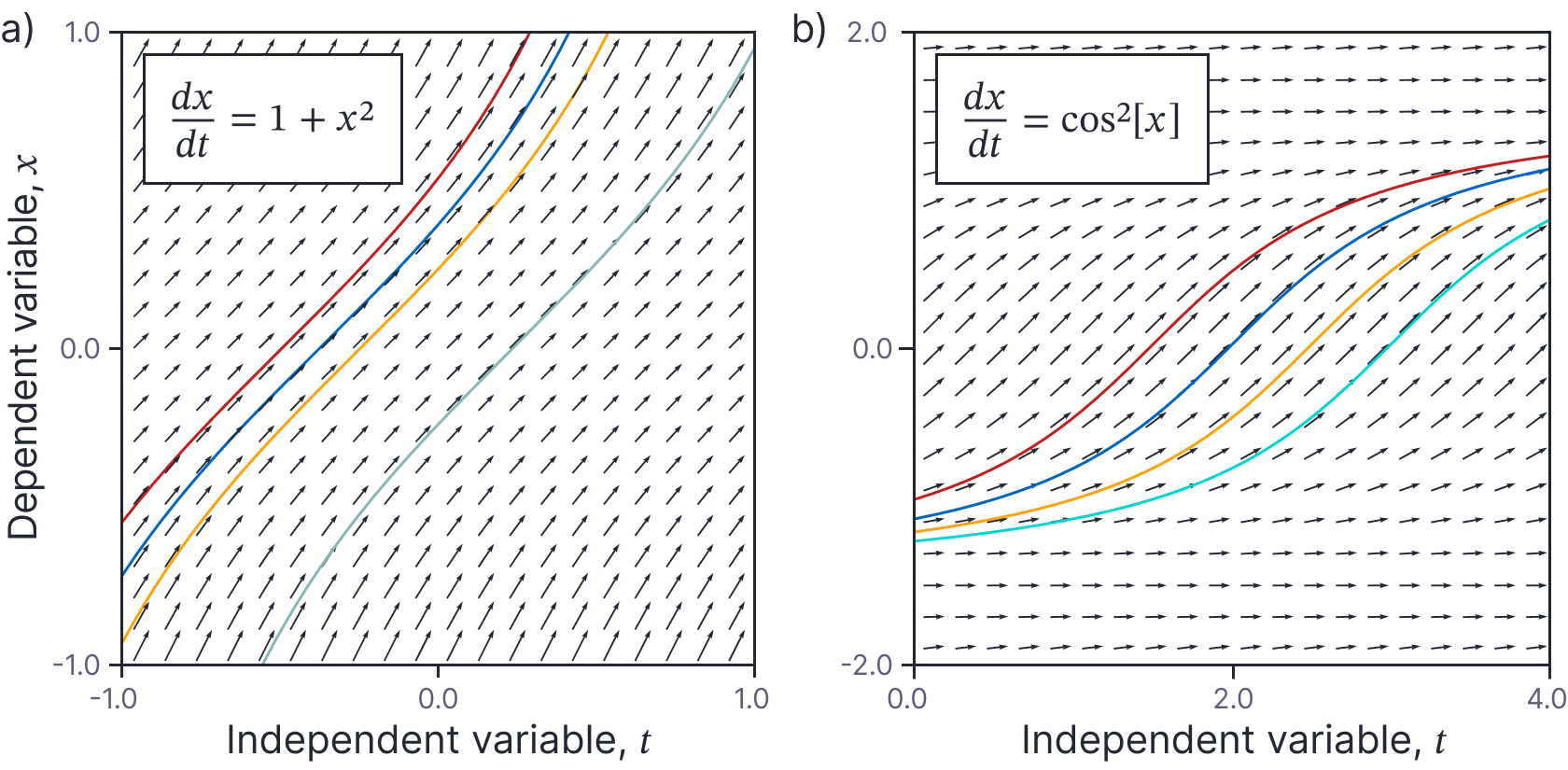
Figure 4. Class 3. Right-hand side is a function of $x$ only. a-b) Two examples. Note that in each case, the flow field is the same at each value of the independent variable $t$ (i.e, the columns of arrows are all identical). The solutions are shifted horizontally relative to one another in this plot, indicating time-invariance.
Solution: The method of solution is similar to that for linear homogeneous ODEs. We move all terms in $x$ to the left-hand side:
\begin{equation}
\frac{1}{\textrm{g}[x]}\frac{dx}{dt}= 1
\tag{30}
\end{equation}
and integrate both sides with respect to $t$, to get:
\begin{equation}\label{eq:ode2_x_only_soln}
\int \frac{1}{\textrm{g}[x]} \frac{dx}{dt} dt = t + C,
\tag{31}
\end{equation}
The solution to the integral on the left-hand side will be a function $\textrm{h}[x]$ whose derivative with respect to $x$ is $1/\textrm{g}[x]$ so that:
\begin{equation}
\frac{dh}{dt} = \frac{dh}{dx}\frac{dx}{dt} = \frac{1}{\textrm{g}[x]} \frac{dx}{dt},
\tag{32}
\end{equation}
and so the solution is:
\begin{equation}\label{eq:ode2_x_only_soln2}
\int \frac{1}{\textrm{g}[x]} dx = t + C.
\tag{33}
\end{equation}
Assuming that we can solve this integral, we can re-arrange the resulting solution to get an expression for $x$ as a function of time. We see from the form of the solution that if $x[t]$ is a solution, so is $x[t+C]$. In other words, the solutions are related by a shift in time.
Example: Consider the ODE:
\begin{equation}
\frac{dx}{dt} = \cos^2[x].
\tag{34}
\end{equation}
with boundary condition $x[0]=-1.24904577$. In this case, equation 33 becomes:
\begin{eqnarray}
\int \frac{1}{\cos^2[x]} dx = t + C.
\tag{35}
\end{eqnarray}
Now we use the standard trigonometric integral $\int 1/\cos^2[x]dx=\int\sec^2[x]dx=\tan[x]$ and re-arrange to find the general solution:
\begin{equation}
x = \arctan[t+C],
\tag{36}
\end{equation}
where $C$ is an arbitrary constant. Substituting in the boundary condition $x=-1.24904577$ at $t=0$, we find that $C=3$. It follows that the particular solution is:
\begin{equation}
x = \arctan[t+3].
\tag{37}
\end{equation}
This is the cyan curve in figure 4b.
Class 4: Right-hand side is a separable function of x and t
We can generalize further to equations of the form:
\begin{equation}\label{eq:ode3_separable_form}
\frac{dx}{dt} = \textrm{f}[t]\textrm{g}[x].
\tag{38}
\end{equation}
An example ODE of this type is depicted in figure 5. Note that classes 1-3 were special cases of this family with $\textrm{g}[x]=1$ (class 1), $\textrm{f}[t]=1$ (class 3), and $\textrm{f}[t]=1,\textrm{g}[x]=ax$ (class 2).
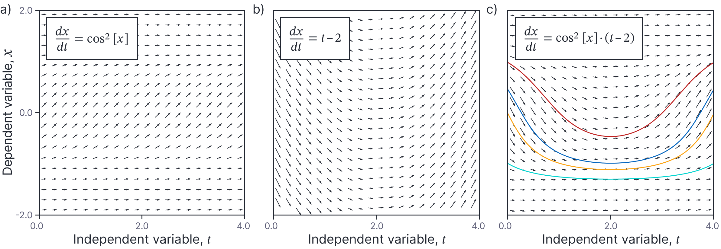
Figure 5. Class 4. right-hand side is a separable function of $x$ and $t$. a) Underlying function of $x$ (gradient field does not vary in horizontal direction). b) Underlying function of $t$ (gradient field does not vary in vertical direction). c) The final ODE is the product of these two flow fields. In general, there is no straightforward relationship between the family of solutions.
Solution: As for the previous two classes of ODE, the solution is found by moving all of the terms in $x$ to the left-hand side and all of the terms in $t$ to the right-hand side:
\begin{equation}
\frac{1}{\textrm{g}[x]}\frac{dx}{dt}= \textrm{f}[t],
\tag{39}
\end{equation}
and then integrating both sides with respect to $t$:
\begin{equation}\label{eq:ode2_separable_soln}
\int \frac{1}{\textrm{g}[x]}dx = \int \textrm{f}[t]dt,
\tag{40}
\end{equation}
where the left-hand side is converted to an integral in $x$ using exactly the same logic as used in the derivations for the two previous classes of ODEs. Assuming we can find an expression for each of these integrals and the resulting equality can be manipulated to be a function of $x$, we have a closed-form solution. Note that for this class of ODE there is no simple relation like scaling or time-shifting that relates the different particular solutions.
Example: Consider the ODE:
\begin{equation}
\frac{dx}{dt} = (t-2)\cos^2[x].
\tag{41}
\end{equation}
with boundary condition $x[0]=0$. Comparing to equation 38, we see that $\textrm{f}[t]=t-2$ and $\textrm{g}[x]=\cos^2[x]$. Substituting these functions into equation 40, we have:
\begin{equation}
\int \frac{1}{\cos^2[x]}dx = \int (t-2)dt.
\tag{42}
\end{equation}
Integrating both sides, we get:
\begin{equation}
\tan[x] = \frac{t^2}{2}-2t+C,
\tag{43}
\end{equation}
which yields the general solution:
\begin{equation}
x = \arctan\left[\frac{t^2}{2}-2t+C\right].
\tag{44}
\end{equation}
Substituting in the boundary condition $x=0$ at $t=0$, we rearrange to find that $C=0$, so the particular solution is:
\begin{equation}
x = \arctan\left[\frac{t^2}{2}-2t\right].
\tag{45}
\end{equation}
This is the orange curve in figure 5c.
Class 5: Exact ODEs
An ODE is exact if it has the form:
\begin{equation}\label{eq:ode3_exact}
\frac{dx}{dt} = -\left(\frac{\partial \textrm{p}[x,t]}{\partial x}\right)^{-1}\frac{\partial \textrm{p}[x,t]}{\partial t},
\tag{46}
\end{equation}
where $\textrm{p}[x,t]$ is termed the potential function.
Note that all separable equations are by definition exact. For the separable equation:
\begin{eqnarray}
\frac{dx}{dt} &=& \textrm{f}[t] \textrm{g}[x],
\tag{47}
\end{eqnarray}
we have:
\begin{eqnarray}\label{eq:ode3_exact_constraints}
\frac{\partial \textrm{p}[x,t]}{\partial x} &=&-\frac{1}{\textrm{g}[x]}\nonumber\\
\frac{\partial \textrm{p}[x,t]}{\partial t} &=& \textrm{f}[t].
\tag{48}
\end{eqnarray}
and the corresponding potential function $p[x,t]$ is given by:
\begin{equation}
\textrm{p}[x,t] = \int -\frac{1}{\textrm{g}[x]} dx + \int \textrm{f}[t] dt.
\tag{49}
\end{equation}
Solution: To solve an exact equations, we re-arrange equation 46 to the form:
\begin{equation}\label{eq:ode3_exact_rearrange}
\frac{\partial \textrm{p}[x,t]}{\partial x}\frac{dx}{dt} + \frac{\partial \textrm{p}[x,t]}{\partial t} = 0
\tag{50}
\end{equation}
and then note that the left-hand side has the form of the total derivative of the function $\textrm{p}[x,t]$:
\begin{eqnarray}
\frac{d \textrm{p}[x,t]}{d t} &=& \frac{\partial \textrm{p}[x,t]}{\partial x}\frac{\partial x}{\partial t} + \frac{\partial \textrm{p}[x,t]}{\partial t}.
\tag{51}
\end{eqnarray}
It follows that the re-arranged ODE in equation 50 becomes:
\begin{equation}
\frac{d\textrm{p}[x,t]}{dt} = 0,
\tag{52}
\end{equation}
which has solutions:
\begin{equation}
\textrm{p}[x,t] = C,
\tag{53}
\end{equation}
where $C$ is an arbitrary constant. In this case, the function $\textrm{p}[x,t]$ is termed a potential function and the solutions are implicitly described by its isocontours (figure 6).
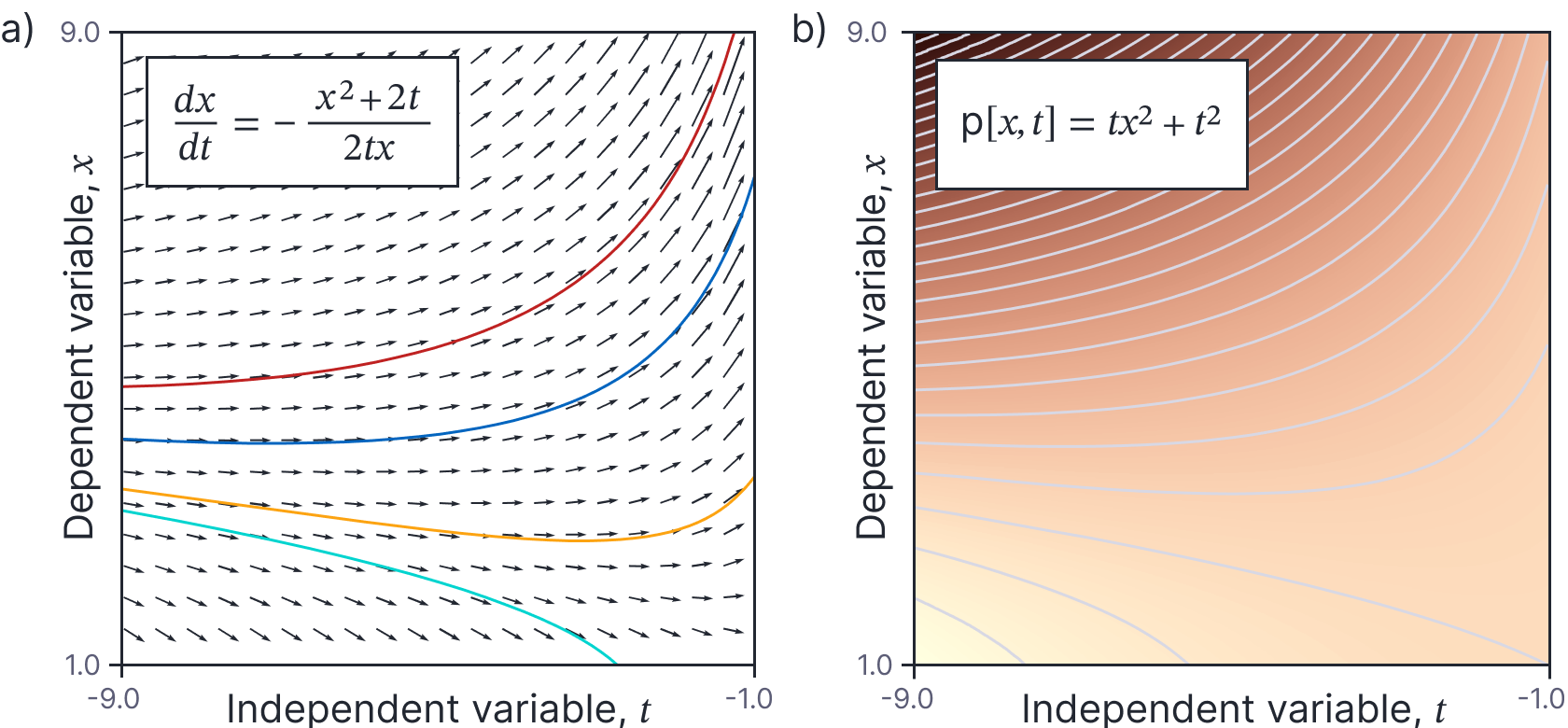
Figure 6. Class 5. Exact ODEs. a) The numerator and denominator of the fraction in the right-hand side are the derivatives with respect to $t$ and $x$ of b) an underlying potential function $\mbox{p}[x,t]$, respectively. Each particular solution of the ODE is an iso-contour (gray lines) of this potential function.
Example: Consider the ODE:
\begin{equation}
\frac{dx}{dt} = -\frac{x^2+2t}{2tx},
\tag{54}
\end{equation}
with boundary conditions $x[-4] = 3$. We can solve this by identifying that it is an exact ODE with potential function:
\begin{equation}
\textrm{p}[x,t] = tx^2+t^2,
\tag{55}
\end{equation}
which has derivatives:
\begin{equation}
\frac{\partial p}{\partial t} = x^2+2t \hspace{1cm}\textrm{and}\hspace{1cm} \frac{\partial p}{\partial x} = 2tx,
\tag{56}
\end{equation}
as required. It follows that the solutions of the ODE are the isocontours of $p[x,t]$ (see figure 6) and the general solution is:
\begin{equation}\label{eq:ode3_example_soln_implicit}
tx^2+t^2 = C
\tag{57}
\end{equation}
which can be re-arranged to yield:
\begin{equation}
x = \pm \sqrt{\frac{C-t^2}{t}}
\tag{58}
\end{equation}
Substituting in the boundary condition $x=3$ at $t=-4$, we find $C=-50$ and the particular solution is:
\begin{equation}
x = \pm \sqrt{\frac{-50-t^2}{t}}.
\tag{59}
\end{equation}
The positive root of this equation corresponds to the dark blue line in figure 6a.
Class 6: linear inhomogeneous ODEs
Consider a linear ODE with the form:
\begin{equation}\label{eq:ode3_linear_inhomogeneous_form}
\frac{dx}{dt} = a x + \textrm{f}[t],
\tag{60}
\end{equation}
where $a$ is a constant and the driving term $\mbox{f}[t]$ is a function of time alone. This is a linear inhomogeneous ODE. It is linear because all terms are proportional to $x$ and its derivatives or are functions of $t$ alone. It is inhomogeneous because of the driving term. However, the right-hand side is not a separable function of $x$ and $t$, nor is it an exact ODE, so it’s not obvious how to proceed.
Solution: To make progress, we seek a transformation of the dependent variable $x$ to a new variable $v$, such that the new ODE becomes solvable using one of our existing methods. Then we solve the ODE in $v$ and transform back to the original dependent variable $x$ to find the solution (figure 7).

Figure 7. Class 6. Linear inhomogeneous ODEs. a) To solve this class of equation, we transform the dependent variable from $x$ to $v=\exp[at]x$. Constant values of the new variable in the original coordinate space are shown. b) When we transform to the variable $v$, these become straight horizontal lines, and the right-hand side of the new equation now only depends on $t$. c) We solve this in the new space (four solutions shown), and then transform back to the original space to get the solutions to the original ODE.
For this equation a suitable change of variable is:
\begin{equation}
v = \exp[-at]x,
\tag{61}
\end{equation}
which implies in turn that:
\begin{equation}\label{eq:ode_lin_inhomog_transform}
x=\exp[at] v,
\tag{62}
\end{equation}
and
\begin{equation}
\frac{dx}{dt} = \exp[at] \frac{dv}{dt} + a\exp[at] v.
\tag{63}
\end{equation}
Now we substitute these expressions into the original ODE (equation 60):
\begin{eqnarray}
\exp[at] \frac{dv}{dt} + a\exp[at] v = a \exp[at] v +\textrm{f}[t],
\tag{64}
\end{eqnarray}
which we simplify to:
\begin{equation}
\frac{dv}{dt} = \exp[-at]\textrm{f}[t].
\tag{65}
\end{equation}
This is an ODE where the right-hand side is a function of $t$ only (i.e., a class 1 ODE). We now solve this equation
\begin{equation}
v = \int\exp[-at] \mbox{f}[t] dt,
\tag{66}
\end{equation}
and transferring back to the original coordinate system using equation 62, we have:
\begin{equation}
x = \exp[at] \int\exp[-at] \mbox{f}[t] dt .
\tag{67}
\end{equation}
This is sometimes described as the “integrating factor” method, although it is really a special case of the more general approach of changing the variable.
Example: Consider the ODE:
\begin{equation}
\frac{dx}{dt} = -\frac{x}{2} + \frac{t}{5},
\tag{68}
\end{equation}
with boundary condition $x[0]=1/5$. This has the form of equation 60 with $a=-1/2$ and $\textrm{f}[t]=t/5$ (see figure 7). According to equation 18, the solution will be:
\begin{equation}
x = \exp\left[-\frac{t}{2}\right]\cdot \int \exp\left[\frac{t}{2}\right]\cdot \frac{t}{5} dt.
\tag{69}
\end{equation}
The integral on the right can be solved using integration by parts which gives the general solution:
\begin{eqnarray}
x &=& \exp\left[-\frac{t}{2}\right]\cdot \left(\frac{2}{5}t\cdot \exp\left[\frac{t}{2}\right] – \frac{4}{5} \exp\left[-\frac{t}{2}\right]+C\right)\nonumber \\
&=& \frac{2}{5}t – \frac{4}{5} + C\exp\left[-\frac{t}{2}\right].
\tag{70}
\end{eqnarray}
where $C$ is the arbitrary integration constant. Substituting in the boundary condition $x=1/5$ at $t=0$, we find that $C=1$, giving the particular solution:
\begin{equation}
x = \frac{2}{5}t – \frac{4}{5} + \exp\left[-\frac{t}{2}\right],
\tag{71}
\end{equation}
which corresponds to the dark blue line in figure 7d.
Class 7: Euler homogeneous
Consider an ODE that can be expressed as:
\begin{equation}
\frac{dx}{dt} = \textrm{h}\left[\frac{x}{t}\right].
\tag{72}
\end{equation}
This is an Euler homogeneous ODE. To make progress, we make a change of variable $v = x/t$. This can be rearranged as $x=v\cdot t$ which implies by the chain rule that:
\begin{equation}
\frac{dx}{dt} = \frac{dv}{dt} t + v.
\tag{73}
\end{equation}
Now we return to the original equation, replacing the terms of the left- and right-hand sides with the new expressions in $v$.
\begin{equation}
\frac{dv}{dt} t + v = \textrm{h}\bigl[v\bigr]
\tag{74}
\end{equation}
We can re-arrange this to:
\begin{equation}\label{eq:ode2_nonlin_homo_soln}
\frac{dv}{dt} = \frac{1}{t}\cdot \Bigl(\textrm{h}\bigl[v\bigr] – v\Bigr),
\tag{75}
\end{equation}
and we now see that this is a separable equation of the type that we already know how to solve. After solving, the equation, we return to the original variable by substituting back in $v=x/t$ (figure 8).
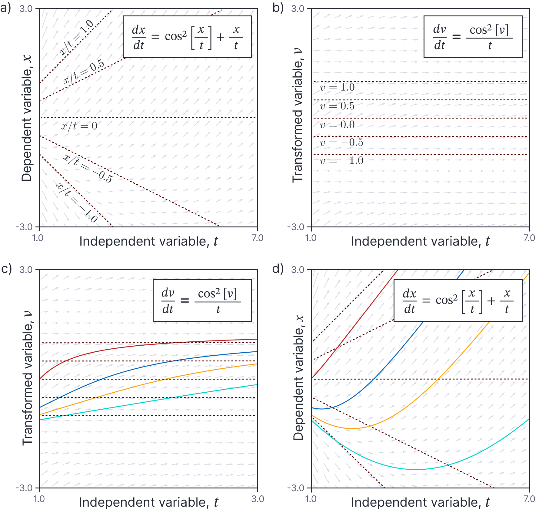
Figure 8. Class 7. Euler homogeneous ODEs. a) To solve this class of equation, we change the dependent variable from $x$ to $v=x/t$. Constant values of the new variable in the original coordinate space are shown. b) When we transform to the variable $v$, these become straight horizontal lines, and the right-hand side of the new equation is now a separable function of $x$ and $t$. c) We solve this in the new space (four solutions shown), and then transform back to the original space to solve the original ODE.
Example: Consider the ODE:
\begin{equation}
\frac{dx}{dt} = \cos^2\left[\frac{x}{t}\right]+\frac{x}{t},
\tag{76}
\end{equation}
with boundary conditions $x[1]=-1.06369782$. Now, we change variables to $v=x/t$ and exploit the solution in equation 75 which yields:
\begin{eqnarray}
\frac{dv}{dt} &=&\frac{1}{t}\cdot \Bigl(\cos^2\left[v\right]+v- v\Bigr)\nonumber \\
&=& \frac{1}{t}\cdot \Bigl(\cos^2\left[v\right]\Bigr).
\tag{77}
\end{eqnarray}
This can be solved using the separation of variables method to yield:
\begin{equation}
\tan[v] = \log[t] + C,
\tag{78}
\end{equation}
where $C$ is an arbitrary constant. This can be re-arranged to:
\begin{equation}
v = \arctan\Bigl[\log[t]+C\Bigr].
\tag{79}
\end{equation}
Substituting back in $v=x/t$ and rearranging, we have the general solution:
\begin{equation}
x = t\cdot \arctan\Bigl[\log[t]+C\Bigr],
\tag{80}
\end{equation}
and using the boundary condition $x=-1.06369782$ when $t=0$, we find $C=-1.8$, giving the particular solution:
\begin{equation}
x = t\cdot \arctan\Bigl[\log[t]-1.8\Bigr],
\tag{81}
\end{equation}
which is the orange curve in figure 8d.
Closed-form solutions for vector ODEs
The previous section described solutions for seven different classes of ODE where the variable $x\in\mathbb{R}$ was scalar. However, in machine learning, the dependent variable $\mathbf{x}\in\mathbb{R}^{D}$ usually describes the parameters, or the data itself and so is vector valued. Fortunately, the basic principles described in the previous section apply to vector ODEs. We’ll look into two cases in detail:
1. Linear homogeneous:
\begin{equation}
\frac{d\mathbf{x}}{dt} = \mathbf{A}\mathbf{x},
\tag{82}
\end{equation}
2. Linear inhomogeneous:
\begin{equation}
\frac{d\mathbf{x}}{dt} = \mathbf{A}\mathbf{x} + \mathbf{B}\textbf{f}[t],
\tag{83}
\end{equation}
where $\textbf{f}[t]$ is a function of the independent variable $t$ that returns a vector and $\mathbf{A}$ and $\mathbf{B}$ are known matrices.
The matrix exponential
Before we can tackle these vector ODEs, we need to introduce the matrix exponential. This is a function $\textbf{Exp}[\mathbf{A}]$ that takes a matrix $\mathbf{A}\in\mathbb{R}^{D\times D}$ and returns another matrix of the same size. Just as the standard exponential is defined by the power series:
\begin{equation}
\exp[a] = 1+ a + \frac{a^2}{2!} + \frac{a^3}{3!}+\ldots,
\tag{84}
\end{equation}
so the matrix exponential is defined by the power series:
\begin{equation}
\textbf{Exp}\bigl[\mathbf{A}\bigr] = \mathbf{I}+ \mathbf{A} + \frac{\mathbf{A}^2}{2!}+ \frac{\mathbf{A}^3}{3!}+\ldots .
\tag{85}
\end{equation}
Note that it is not the same as independently exponentiating the terms in the matrix argument.
In general, the matrix exponential is difficult to calculate by hand, but there are some special cases where this is easy:
Identity matrix: If $\mathbf{A}=\mathbf{I}$, then the matrix exponential is a diagonal matrix with the natural number $e$ on each element of the diagonal:
\begin{equation}
\textbf{Exp}\Biggl[\begin{bmatrix}1 &0 \\ 0 & 1\end{bmatrix} \Biggr] =\mathbf{I}+ \mathbf{I} + \frac{\mathbf{I}}{2!}+ \frac{\mathbf{I}}{3!}+\ldots = \begin{bmatrix} e & 0 \\0 & e \end{bmatrix}.
\tag{86}
\end{equation}
Diagonal matrix: If $\mathbf{A}$ is diagonal with $a_k$ on the $k^{th}$ diagonal, then the matrix exponential is a diagonal matrix with $e^{a_{k}}$ on the $k^{th}$ diagonal:
\begin{eqnarray}
\textbf{Exp}\Biggl[\begin{bmatrix}a_1 &0 \\ 0 & a_2\end{bmatrix} \Biggr] &=&\mathbf{I}+ \begin{bmatrix}a_1 &0 \\ 0 & a_2 \end{bmatrix} + \frac{1}{2!}\begin{bmatrix}a_1^2 &0 \\ 0 & a_2^2\end{bmatrix} + \frac{1}{3!}\begin{bmatrix}a_1^3 &0 \\ 0 & a_2^3\end{bmatrix} +\ldots \nonumber \\
&=& \begin{bmatrix} e^{a_1} & 0 \\0 & e^{a_2} \end{bmatrix}.
\tag{87}
\end{eqnarray}
Diagonalizable matrix: If $\mathbf{A}$ is diagonalizable as $\mathbf{P}\mathbf{D}\mathbf{P}^{-1}$ where $\mathbf{P}$ is an orthogonal matrix containing the eigenvectors in its columns, $\mathbf{P}^{-1}=\mathbf{P}^{T}$ and $\mathbf{D}$ is a diagonal matrix containing the eigenvalues, then $\textbf{Exp}[\mathbf{A}] = \mathbf{P}\textbf{Exp}[\mathbf{D}]\mathbf{P}^T$:
\begin{eqnarray}
\textbf{Exp}\bigl[\mathbf{A}\bigr] &=& \mathbf{I}+ \mathbf{A} + \frac{\mathbf{A}^2}{2!}+ \frac{\mathbf{A}^3}{3!}+\ldots \nonumber \\
&=& \mathbf{I} + \mathbf{P}\mathbf{D}\mathbf{P}^{-1}+ \frac{\mathbf{P}\mathbf{D}^2\mathbf{P}^{-1}}{2!}+ \frac{\mathbf{P}\mathbf{D}^3\mathbf{P}^{-1}}{3!}+\ldots \nonumber \\
&=& \mathbf{P}\left(\mathbf{I} + \mathbf{D}+ \frac{\mathbf{D}^2}{2!}+ \frac{\mathbf{D}^3}{3!}+\ldots\right)\mathbf{P}^{-1} \nonumber \\
&=& \mathbf{P}\textbf{Exp}[\mathbf{D}]\mathbf{P}^{-1}.
\tag{88}
\end{eqnarray}
Nilpotent matrix: If $\mathbf{A}$ is a nilpotent matrix of order $K$ to that $\mathbf{A}^K=0$, then we can truncate the power series at index $K-1$. For example, if $\mathbf{A}^2=\mathbf{0}$:
\begin{eqnarray}
\textbf{Exp}\bigl[\mathbf{A}\bigr] &=& \mathbf{I}+ \mathbf{A} + \frac{\mathbf{A}^2}{2!}+ \frac{\mathbf{A}^3}{3!}+\ldots \nonumber \\
&=& \mathbf{I}+ \mathbf{A} + \frac{\mathbf{0}}{2!}+ \frac{\mathbf{A}\mathbf{0}}{3!}+\ldots \nonumber \\
&=& \mathbf{I}+ \mathbf{A}.
\tag{89}
\end{eqnarray}
Sum of commutative matrices: If $\mathbf{A}$ and $\mathbf{B}$ commute so that $\mathbf{A}\mathbf{B}=\mathbf{B}\mathbf{A}$ then $\textbf{Exp}[\mathbf{A}+\mathbf{B}]=\textbf{Exp}[\mathbf{A}]\textbf{Exp}[\mathbf{B}]$. To show this, we first write out the expansions of each matrix:
\begin{eqnarray}
\textbf{Exp}\bigl[\mathbf{A}\bigr] &=& \mathbf{I}+ \mathbf{A} + \frac{\mathbf{A}^2}{2!}+ \frac{\mathbf{A}^3}{3!}+\ldots \nonumber \\
\textbf{Exp}\bigl[\mathbf{B}\bigr] &=& \mathbf{I}+ \mathbf{B} + \frac{\mathbf{B}^2}{2!}+ \frac{\mathbf{B}^3}{3!}+\ldots
\tag{90}
\end{eqnarray}
Then we multiply the two series together:
\begin{eqnarray}
\textbf{Exp}\bigl[\mathbf{A}\bigr] \textbf{Exp}\bigl[\mathbf{B}\bigr]& =& \mathbf{I}+\mathbf{A}+\mathbf{B}+\frac{\mathbf{A}^2}{2!}+\mathbf{A}\mathbf{B}+\frac{\mathbf{B}^2}{2!}+\ldots\nonumber \\
& =& \mathbf{I}+\mathbf{A}+\mathbf{B}+\frac{\mathbf{A}^2}{2!}+\frac{2\mathbf{A}\mathbf{B}}{2!}+\frac{\mathbf{B}^2}{2!}+\ldots\nonumber \\
& =& \mathbf{I} + \mathbf{A}+\mathbf{B} + \frac{\mathbf{A}^2+\mathbf{A}\mathbf{B}+\mathbf{B}\mathbf{A}+\mathbf{B}^2}{2!}+\ldots\nonumber\\
& =& \mathbf{I} + (\mathbf{A}+\mathbf{B}) + \frac{(\mathbf{A}+\mathbf{B})^2}{2!}+\ldots\nonumber\\
& =& \textbf{Exp}[\mathbf{A}+\mathbf{B}],
\tag{91}
\end{eqnarray}
where we have used the commutative property between lines 2 and 3, to write $ 2\mathbf{A}\mathbf{B}=\mathbf{A}\mathbf{B}+\mathbf{B}\mathbf{A}$. Note that we have only expanded up to terms with denominator $2!$, but the proof continues in the same way for higher-order terms.
Linear homogeneous vector ODEs
Consider the generalization of class 2 (linear homogeneous ODEs) to the case where the dependent variable $\mathbf{x}\in\mathbb{R}^{D}$ is a vector:
\begin{equation}\label{eq:ODE3_vector_homog}
\frac{d\mathbf{x}}{dt} = \mathbf{A} \mathbf{x},
\tag{92}
\end{equation}
and $\mathbf{A}\in\mathbb{R}^{D\times D}$.
Solution: We’ll solve using a slightly different approach to that used in the scalar case as this allows us to derive the matrix exponential along the way. However, both methods work for the scalar and vector cases. We start by integrating both sides of the equation:
\begin{equation}
\int\frac{d\mathbf{x}}{dt} dt= \int \mathbf{A} \mathbf{x} dt.
\tag{93}
\end{equation}
Since the integral of the derivative of $\mathbf{x}$ is just $\mathbf{x}$ itself, it follows that:
\begin{equation}
\mathbf{x} = \mathbf{c} + \int \mathbf{A} \textbf{x} dt,
\tag{94}
\end{equation}
where $\mathbf{c}\in\mathbb{R}^{D}$ is an unknown vector constant. We now substitute this expression for $\mathbf{x}$ into in the right-hand side of its own definition to yield:
\begin{eqnarray}
\mathbf{x} &=& \mathbf{c}+ \int \mathbf{A} \left(\mathbf{c}+ \int \mathbf{A} \mathbf{x} \cdot dt \right)dt\nonumber\\
&=& \mathbf{c}+ \int \mathbf{A} \mathbf{c} \cdot dt+ \int\!\!\int \mathbf{A}^2 \mathbf{x} \cdot dt\cdot dt\nonumber \\
&=& \mathbf{c}+ \mathbf{A}\mathbf{c}\cdot t + \int\!\!\int \mathbf{A}^2 \mathbf{x} \cdot dt\cdot dt.
\tag{95}
\end{eqnarray}
Repeating this process, by substituting in for $\mathbf{x}$ we get:
\begin{equation}
\mathbf{x} = \mathbf{c}+ \mathbf{A}\mathbf{c} \cdot t + \mathbf{A}^2 \mathbf{c}\cdot \frac{t^2}{2}+ \int\!\!\int\!\!\int \mathbf{A}^3 \mathbf{x} \cdot dt\cdot dt\cdot dt ,
\tag{96}
\end{equation}
and continuing in this manner yields:
\begin{eqnarray}\label{eq:ode3_vector_homog_soln}
\mathbf{x} &=& \biggl(\mathbf{I}+ \mathbf{A} t + \frac{\mathbf{A}^2t^2}{2!}+ \frac{\mathbf{A}^3t^3}{3!}+\ldots \biggr)\mathbf{c}\nonumber \\
&=& \textbf{Exp}\bigl[\mathbf{A} t\bigr]\mathbf{c},
\tag{97}
\end{eqnarray}
\noindent where the matrix exponential $\textbf{Exp}[\bullet]$ returns a $D\times D$ matrix and is defined as the series in the brackets. Several example solutions of this type of equation are depicted in figure 9. When the matrix $\mathbf{A}$ is diagonal, the two dimensions of the dependent variable don’t interact and exhibit either exponential growth or exponential decay as in figure 3. When the matrix $\mathbf{A}$ has a more general form, the flow pattern can exhibit shearing and rotational patterns.
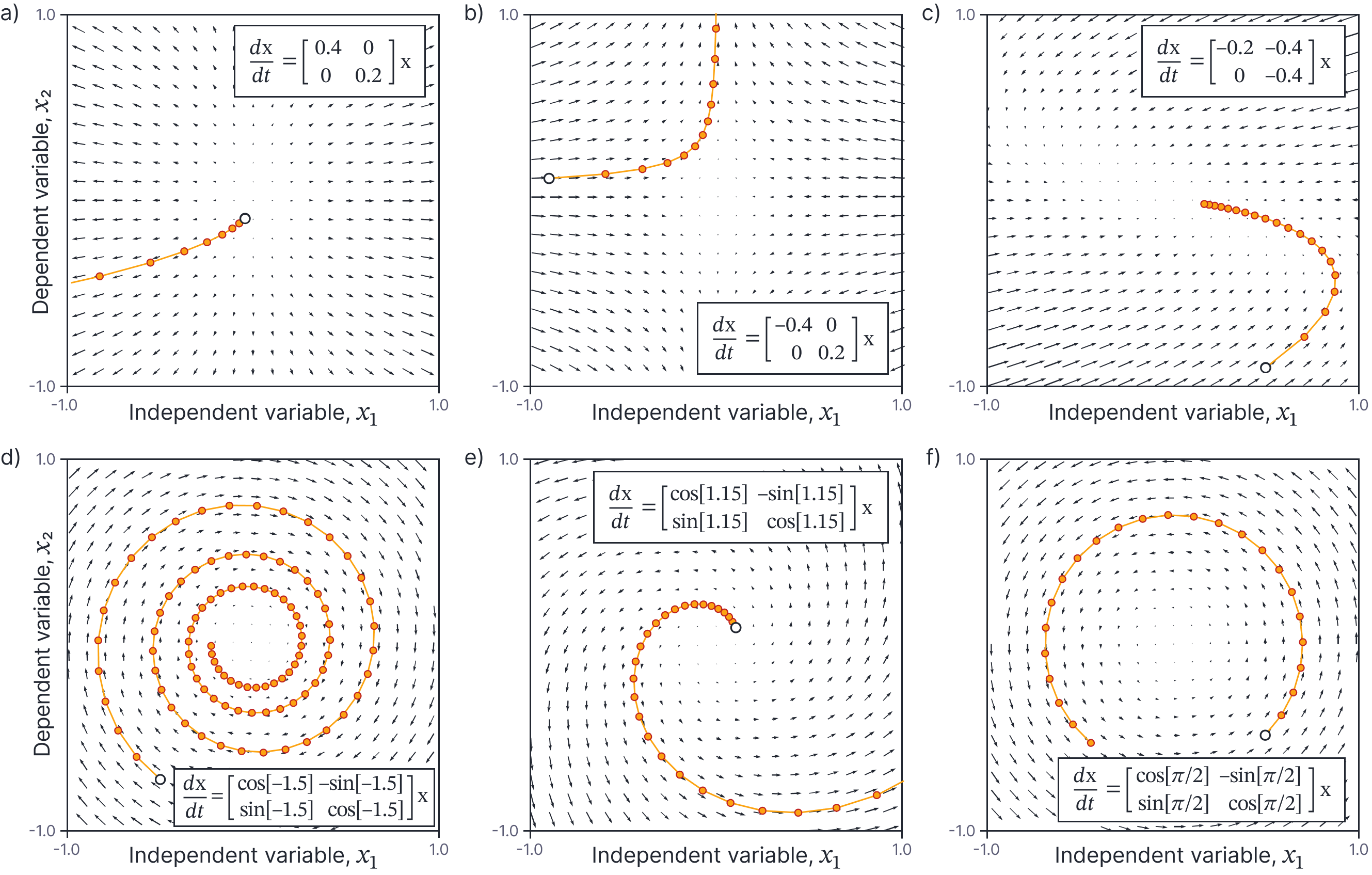
Figure 9. Linear homogeneous vector ODEs. a) Example ODE. The right-hand side does not depend on $t$ and so the vector field showing the change in dependent variable $\mathbf{x}$ is the same at each time-step. The initial point (boundary condition) is depicted by the white circle and the time evolution by the dots along the solution which represent constant time increments of 0.1. In this case, the solution involves exponential growth in the first dimension $x_1$ of $\mathbf{x}$ and slightly slower exponential growth in the second dimension $x_{2}$. b) A second ODE with exponential decay in $x_{1}$ and exponential growth in $x_{2}$. Other choices for $\mathbf{A}$ in equation \ref{eq:ODE3_vector_homog} result in c) shearing patterns in the vector field, and d) rotation that spiral inwards, e) spiral outwards or f) stay at the same radius.
Example: Consider the vector ODE:
\begin{equation}
\frac{d\mathbf{x}}{dt} = \begin{bmatrix}0.4 & 0 \\ 0 & 0.2 \end{bmatrix}\mathbf{x},
\tag{98}
\end{equation}
with boundary condition $\mathbf{x}[0]=[-0.05, -0.1]^T$. Applying equation 97, we find the general solution:
\begin{equation}
\mathbf{x} = \textbf{Exp}\left[\begin{bmatrix}0.4 & 0 \\ 0 & 0.2 \end{bmatrix} t\right]\mathbf{c},
\tag{99}
\end{equation}
where $c$ is an unknown vector constant. If we substitute in the boundary condition $\mathbf{x}=[-0.05, -0.1]$ at time $t=0$, we find that $\mathbf{c}=[-0.05,-0.1]^T$ and get the particular solution
\begin{eqnarray}
\mathbf{x} &=& \textbf{Exp}\left[\begin{bmatrix}0.4 & 0 \\ 0 & 0.2 \end{bmatrix} t\right]\begin{bmatrix}-0.05\\-0.1\end{bmatrix}\nonumber \\
&=& \begin{bmatrix}-0.05 e^{0.4t}\\-0.1 e^{0.2t}\end{bmatrix},
\tag{100}
\end{eqnarray}
where we have used the rules for calculating the matrix exponential of a diagonal matrix between the two lines. This is depicted in figure 9a.
Linear inhomogeneous vector ODEs
Consider the generalization of the linear inhomogeneous ODE (see section 1.8) to a vector variable $\mathbf{x}\in\mathbb{R}^{D}$:
\begin{equation}
\frac{d\textbf{x}}{dt} = \mathbf{A} \mathbf{x} + \mathbf{B} \textbf{f}[t],
\tag{101}
\end{equation}
where the matrices $\mathbf{A}\in \mathbb{R}^{D\times D}$ and $\mathbf{B}\in \mathbb{R}^{D \times D_{f}}$ are constant and the driving term $\textbf{f}[t]$ is some function of time alone that returns a vector of length $D_{f}$. This type of ODE is difficult to visualize; even with $D=2$ there would be 3D volume with a different “arrow” representing the change in $\mathbf{x}$ at each 2D value of the dependent variable $\mathbf{x}$ at each time, $t$.
Solution: This can be solved exactly as for the scalar case, by applying a change of variables $\mathbf{v} = \textbf{Exp}[-\mathbf{A} \mathbf{x}]$ (this time using the matrix exponential). Once more, we solve in this new space, and then transform the solution back to the original variable $x$. After working through the algebra using exactly the same steps as before, we yield the solution:
\begin{equation}\label{eq:ode2_linear_homogeneous_vector_soln}
\mathbf{x} = \textbf{Exp}\bigl[\mathbf{A} t\bigr]\cdot \int \textbf{Exp}\bigl[-\mathbf{A} t\bigr] \mathbf{B} \textbf{f}[t]dt.
\tag{102}
\end{equation}
Example: Consider the linear inhomogeneous vector ODE:
\begin{equation}
\frac{d\textbf{x}}{dt} = \begin{bmatrix}4&4 \\-1 & 0\end{bmatrix} \mathbf{x} + \begin{bmatrix}1\\1\end{bmatrix}\exp[-2t],
\tag{103}
\end{equation}
and boundary conditions $\mathbf{x}[0] = [3,2]^T$. According to equation 102, the general solution to this equation is given by:
\begin{eqnarray}\label{eq:ode3_vector_inhomog_gen_int}
\mathbf{x} = \textbf{Exp}\Biggl[\begin{bmatrix}4 &4 \\ -1 & 0\end{bmatrix} t\Biggr]\cdot \int \textbf{Exp}\Biggl[ -\begin{bmatrix}4 &4 \\ -1 & 0\end{bmatrix} t\Biggr] \begin{bmatrix}1\\1\end{bmatrix}\exp[-2t]dt.
\tag{104}
\end{eqnarray}
To evaluate this equation, we first need to find an expression for the matrix exponential. We can make progress by noting that:
\begin{equation}
\begin{bmatrix}4 &4 \\ -1 & 0\end{bmatrix} = \begin{bmatrix}2 &4 \\ -1 & -2\end{bmatrix} + \begin{bmatrix}2 &0 \\ 0 & 2\end{bmatrix},
\tag{105}
\end{equation}
where the first matrix on the right-hand side is nilpotent of order 2, and the second matrix is diagonal. Moreover, these two matrices commute. Applying the rules from the section on the matrix exponential, we see that:
\begin{eqnarray}
\textbf{Exp}\Biggl[\begin{bmatrix}4 &4 \\ -1 & 0\end{bmatrix}t\Biggr] &=& \textbf{Exp}\Biggl[\begin{bmatrix}2 &4 \\ -1 & -2\end{bmatrix}t + \begin{bmatrix}2 &0 \\ 0 & 2\end{bmatrix}t\Biggr]\nonumber \\
&=& \textbf{Exp}\Biggl[\begin{bmatrix}2 &4 \\ -1 & -2\end{bmatrix}t\Biggr] \textbf{Exp} \Biggl[\begin{bmatrix}2 &0 \\ 0 & 2\end{bmatrix}t\Biggr]\nonumber\\
&=& \begin{bmatrix}1+2t &4t \\ -t & 1-2t\end{bmatrix}\textbf{Exp} \Biggl[\begin{bmatrix}2 &0 \\ 0 & 2\end{bmatrix}t\Biggr]\nonumber \\
&=& \begin{bmatrix}1+2t&4t \\ -t& 1-2t\end{bmatrix}\begin{bmatrix}e^{2t} &0 \\ 0 & e^{2t} \end{bmatrix}\nonumber\\
&=& \begin{bmatrix}e^{2t}+2te^{2t} &4te^{2t} \\ -te^{2t} & e^{2t}-2te^{2t}\end{bmatrix},
\tag{106}
\end{eqnarray}
where we have used the commutative property between lines 1 and 2, the nilpotent property between lines 2 and 3 and the diagonal property between lines 3 and 4 (see previous section).
Substituting this result into the general solution (equation 104), we get:
\begin{eqnarray}
\mathbf{x}&=& \begin{bmatrix}e^{2t}+2te^{2t} &4te^{2t} \\ -te^{2t} & e^{2t}-2te^{2t}\end{bmatrix}\int \begin{bmatrix}e^{2t}+2te^{2t} &4te^{2t} \\ -te^{2t} & e^{2t}-2te^{2t}\end{bmatrix}\begin{bmatrix}1\\1\end{bmatrix}\exp[-2t]dt\nonumber\\
&=& \begin{bmatrix}e^{2t}+2te^{2t} &4te^{2t} \\ -te^{2t} & e^{2t}-2te^{2t}\end{bmatrix}\int \begin{bmatrix}1+6t\\2t\end{bmatrix}dt\nonumber\\
&=& \begin{bmatrix}e^{2t}+2te^{2t} &4te^{2t} \\ -te^{2t} & e^{2t}-2te^{2t}\end{bmatrix}\begin{bmatrix}t+3t^2+C_1\\t^2+C_2\end{bmatrix}\nonumber\\
&=& \begin{bmatrix}(e^{2t}+2te^{2t})(t+3t^2+C_1)+ 4e^{2t}(t^2+C_2) \\-te^{2t}(t+3t^2+C_1)+(e^{2t}-2te^{2t})(t^2+C2)\end{bmatrix}.
\tag{107}
\end{eqnarray}
Finally, we can substitute in the boundary condition $\mathbf{x} = [3,2]^T$ when $t=0$, to find that $C_{1}=-1$ and $C_{2}=1$:
\begin{equation}
\mathbf{x}= \begin{bmatrix}(e^{2t}+2te^{2t})(t+3t^2-1)+ 4e^{2t} \\e^{2t}(-t-3t^2)\end{bmatrix}.
\tag{108}
\end{equation}
Discussion
This article described a family of approaches to finding closed-form expressions for first-order ODEs. The main part of the article dealt with the scalar case, but we also consider vector ODEs for the linear homogeneous and linear inhomogeneous cases. The details of these solutions are more complicated, but the principles are the same. Of course, higher-order ODEs can be converted to vector ODEs (see part II of this series) and so this also opens a window to solve these too.
Unfortunately, there are still many ODEs that cannot be solved in closed form. For these, we use numerical methods; we start with the initial boundary condition and iteratively move the solution forward in time by evaluating the gradient using the ODE. These methods will be described in the next article in this series.