
In part III of this series of articles, we discussed closed-form solutions to ordinary differential equations (ODEs) and developed methods to derive an equation for the general solution of an ODE. This solution represents the family of all functions that obey the ODE. By imposing boundary conditions, we can determine a particular solution (one member of this family) which is a single trajectory through the ODE. In this article (part IV of the series) we consider the many ODEs for which there is no known technique to find a closed-form solution; both the individual members of this family, and the relationship between them can be complicated (figure 1).
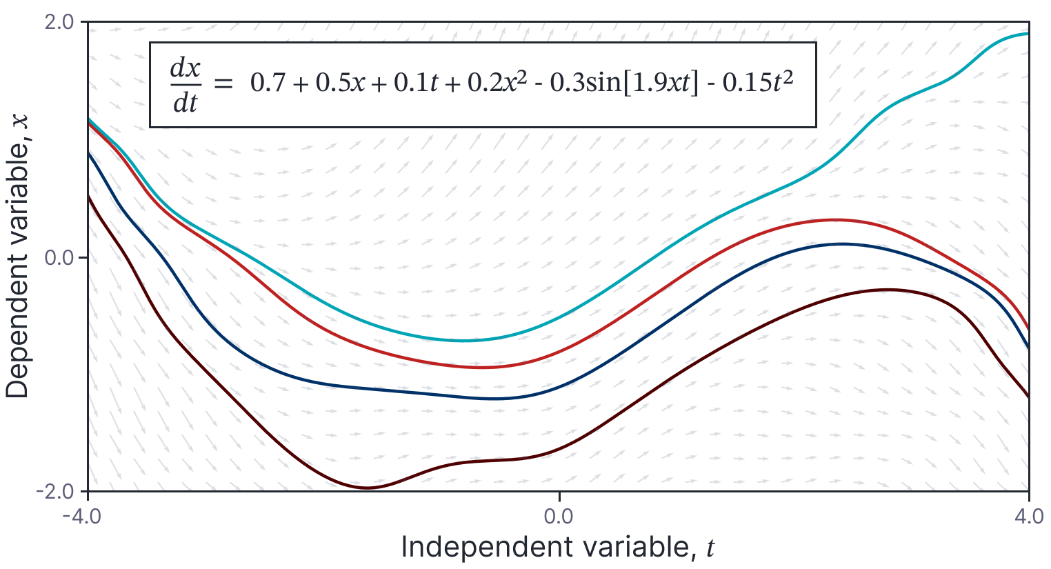
Figure 1. Example ODE and solutions. The ODE os represented as a direction field. For each value of $t$ (abscissa) and $x$ (ordinate), the derivative $dx/dt$ is represented as an arrow. If the derivative is zero then arrow will be horizontal. If it is positive, it will be oriented upwards and if it is negative, it will be oriented downwards. The four lines depict four of the many possible solutions to the equation. Each line follows the arrows in the direction field along its path. In this case, each solution is a complicated function and the relationships between the solutions are not straightforward.
When faced with a differential equation that we cannot solve, we turn to numerical methods. In the simplest case, we start with an initial condition (e.g., $x=3$ at $t=0$) and propagate this solution forward; we alternately (i) evaluate the ODE to determine how the function is changing at the current position and (ii) use this information to predict where the solution will be shortly thereafter.
This article will describe many variations of this scheme which trade off accuracy against efficiency. We will concentrate on first-order equations where the dependent variable $x\in\mathbb{R}$ is scalar. However, as we shall see, these techniques can easily be adapted to vector valued variables $\mathbf{x}\in\mathbb{R}^{D}$.
This article is accompanied by a Python notebook that reproduces the results.
Numerical solutions
Consider a first-order ordinary differential equation of the form:
\begin{equation}
\frac{d\textrm{x}[t]}{dt} = \textrm{f}\bigl[\textrm{x}[t], t\bigr],
\tag{1}
\end{equation}
with initial boundary condition $\textrm{x}[t_{0}]$. If we cannot find a closed-form solution for $\textrm{x}[t]$, we can still compute a numerical estimate of the particular solution $\textrm{x}[t_n]$ at time steps $t_{n} = t_{0}+nh$, where $h$ is the step size and $n\in[1,2,3,\ldots]$:
\begin{eqnarray}
\textrm{x}[t_{0}+h] &=& \textrm{x}[t_{0}] + \int_{t_0}^{t_0+h} \textrm{f}\bigl[\textrm{x}[\tau],\tau\bigr] d\tau\nonumber \\
\textrm{x}[t_{0}+2h] &=& \textrm{x}[t_{0}+h] + \int_{t_0+h}^{t_0+2h} \textrm{f}\bigl[\textrm{x}[\tau],\tau\bigr] d\tau\nonumber \\
\textrm{x}[t_{0}+3h] &=& \textrm{x}[t_{0}+2h] + \int_{t_0+2h}^{t_0+3h} \textrm{f}\bigl[\textrm{x}[\tau],\tau\bigr] d\tau,
\tag{2}
\end{eqnarray}
and so on. This yields a series of points which (hopefully) lie along the trajectory of the true solution. This process was used to create figure 1 and the “curves” in this figure actually comprise a series of points at intervals $h = 0.01$ that have been connected by straight lines for visualization.
Two simple methods
How should we estimate these integrals? A starting point is to consider how we might numerically integrate a standard function (ie, not an ODE). Two standard methods (figure 2) are forward Euler integration (in which we divide the function to be integrated into rectangular regions of width $h$ and sum the area of these regions) and trapezoidal integration (which uses trapezoidal regions). The next two subsections describe two methods for numerical approximation of ODEs that are inspired by the forward Euler and trapezoidal integration methods, respectively.
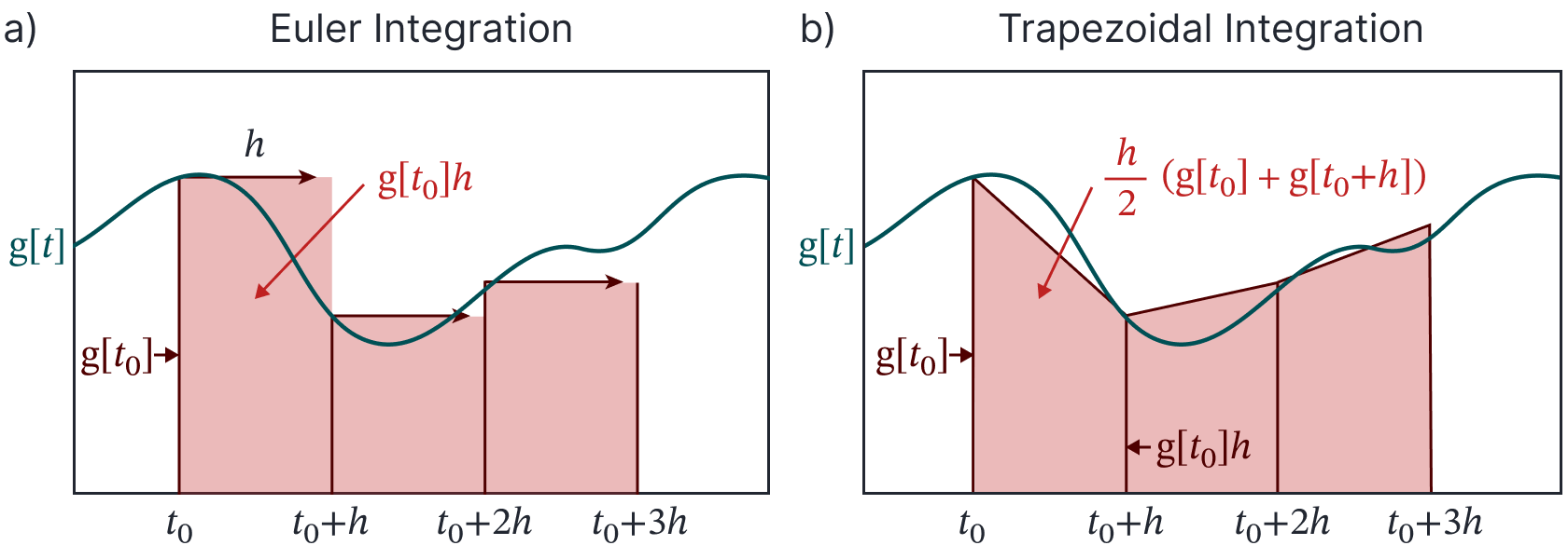
Figure 2. Numerical integration of a standard function $\mbox{g}[t]$ (not an ODE). a) Forward Euler integration. We calculate the area under the curve with a series of rectangular approximations; each rectangular area is computed by multiplying the height of the function $\mbox{g}[t]$ at the current time by the step size $h$. b) Trapezoidal method. A better approximation to the area under the curve can be estimated by dividing it into trapezoids; the area of each trapezoid is computed by taking the average of the heights of the function $\mbox{g}[t]$ and $\mbox{g}[t+h]$ at the start and end of the region and multiplying this average by the step size $h$.
Euler method
The simplest numerical approach to ODEs is the Euler method, which is equivalent to the Euler integration method for standard functions. The Euler method approximates the integral as the area of a rectangle of height $\textrm{f}\bigl[\textrm{x}[t],t\bigr]$ and width $h$:
\begin{equation}\label{eq:ODE4_Euler_integral}
\int_{t}^{t+h} \textrm{f}\bigl[\textrm{x}[\tau],\tau\bigr] d\tau\approx \textrm{f}\bigl[\textrm{x}[t],t\bigr]h.
\tag{3}
\end{equation}
In practice, this means that we compute the numerical solution to the ODE by iterating:
\begin{equation}
\textrm{x}[t+h] = \textrm{x}[t] + \textrm{f}\bigl[\textrm{x}[t],t\bigr]h.
\tag{4}
\end{equation}
This is easy to understand in terms of the output function $\textrm{x}[t]$; it is equivalent to projecting the function forward based on the gradient at the current point $t$ for a distance $h$ (figure 3a).
Just as for Euler integration, this accrues an error at each step; the derivative $\textrm{f}\bigl[\textrm{x}[t],t\bigr]$ at the current point on the solution does not necessarily capture all of the variation in the region $[t,t+h]$. However, the situation is worse for ODEs; not only do we accrue an error at the first step, but the starting point for the next step $\textrm{x}[t_0+h]$ is now wrong, so the derivative $\textrm{f}\bigl[\textrm{x}[t+h],t+h\bigr]$ will also be wrong.
In this way, we can gradually diverge from the true path of the ODE (figure 3b). This problem can reduced when we use smaller step sizes, but of course we pay a price in terms of increased computation.
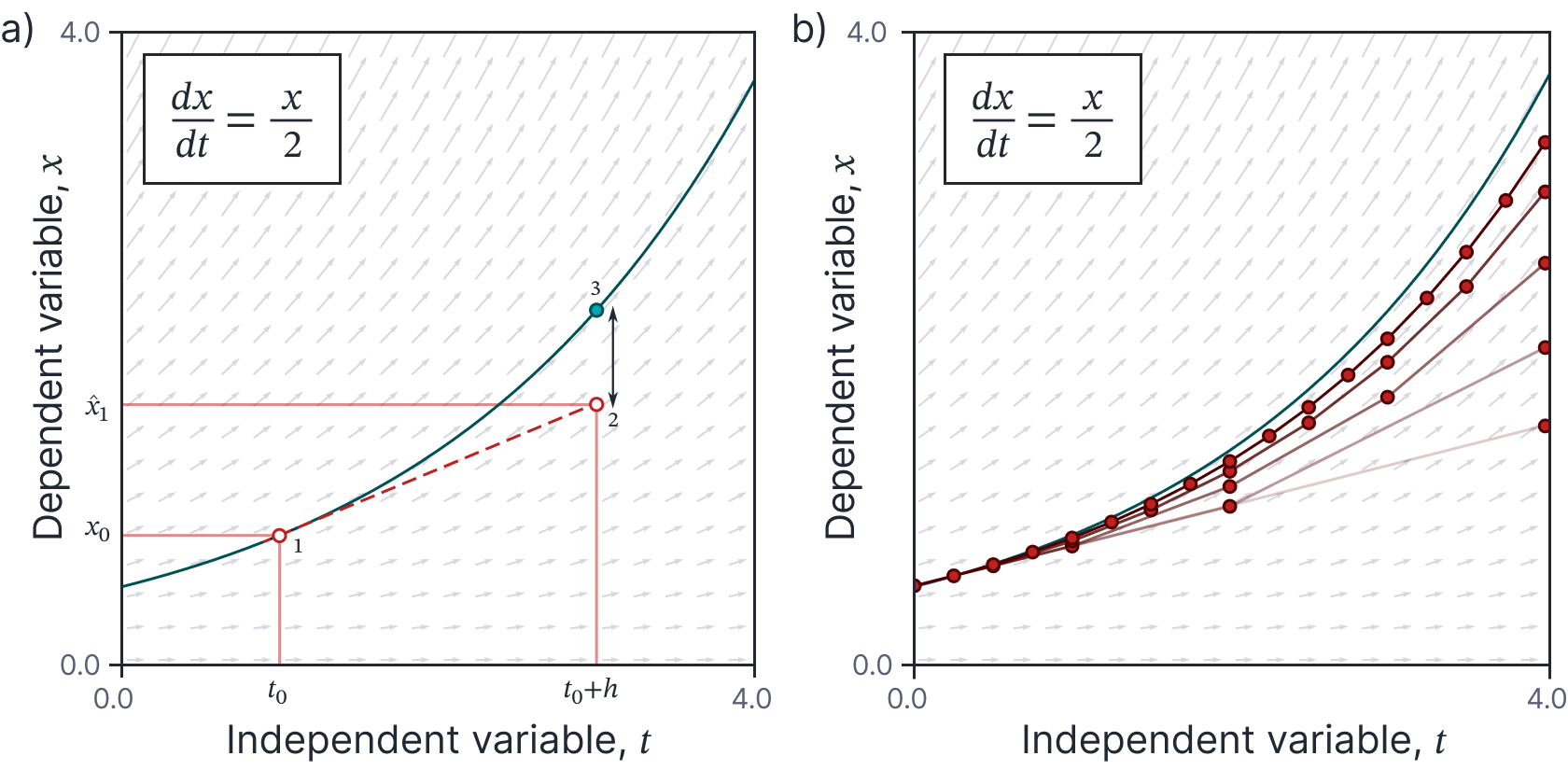
Figure 3. Euler method. a) We start at the initial boundary condition at time $t_0$ and initial condition $x_{0}$ (point 1), and evaluate the ODE to measure the gradient at this point. We use this gradient to project forward to point 2 at time $t_1=t_0+h$ and estimate the corresponding value $x_{1}$. With a large step size $h$, this linear approximation deviates significantly from the true value (point 3) of the function at time $t_1$. The deviation between this numerical solution and closed-form solution (green curve) will increase over time, not least because the derivative for the next step will be taken at the wrong place. b) However, as the step size $h$ decreases, the cumulative error decreases and the numerical solution approaches the ground truth. The five brown curves represent numerical approximations with step sizes $h=4,2,1,0.5$, and $0.25$. This pattern of curves is sometimes referred to as Lady Windermere’s Fan after the Oscar Wilde play of the same name.
Heun’s method
Now let’s consider the ODE equivalent of trapezoidal integration (figure 2):
\begin{equation}
\int_{t}^{t+h} \textrm{f}\bigl[\textrm{x}[\tau],\tau\bigr] d\tau\approx \frac{h}{2}\Bigl( \textrm{f} \bigl[\textrm{x}[t],t\bigr]+\textrm{f}\bigl[\textrm{x}[t+h],t+h\bigr]\Bigr),
\tag{5}
\end{equation}
which takes the area under the curve as the width $h$ on the interval multiplied by the average of the values $\textrm{f} \bigl[\textrm{x}[t],t\bigr]$ and $\textrm{f}\bigl[\textrm{x}[t+h],t+h\bigr]$ at the start and the end of the interval, respectively.
However, we can’t easily compute this, as we don’t know the value of $\textrm{x}[t+h]$ — this is what we are trying to compute in the first place. Heun’s method approximates this value with the its estimate $\textrm{x}[t+h]\approx \textrm{x}_{t}+\textrm{f}\bigl[\textrm{x}[t],t\bigr]h$ from a single Euler step:
\begin{equation}
\int_{t}^{t+h} \textrm{f}\bigl[\textrm{x}[\tau],\tau\bigr] d\tau\approx \frac{h}{2}\Bigl( \textrm{f} \bigl[\textrm{x}[t],t\bigr]+
\textrm{f}\Bigl[\color{red}\textrm{x}[t]+\textrm{f}\bigl[\textrm{x}[t],t\bigr]h\color{black},t+h\Bigr]\Bigr).
\tag{6}
\end{equation}
Hence, Heun’s method consists of iterating:
\begin{equation}
\textrm{x}[t+h] = \textrm{x}[t] + \frac{h}{2}\Bigl( \textrm{f} \bigl[\textrm{x}[t],t\bigr]+
\textrm{f}\Bigl[\textrm{x}[t]+\textrm{f}\bigl[\textrm{x}[t],t\bigr]h,t+h\Bigr]\Bigr).
\tag{7}
\end{equation}
In terms of the solution $\textrm{x}[t]$ this is equivalent to (i) projecting forward from the initial point using the gradient at the current point, (ii) measuring the gradient at this predicted point (iii) projecting forward from the initial point again using this new gradient and (iv) averaging these two predictions together (figure 4).
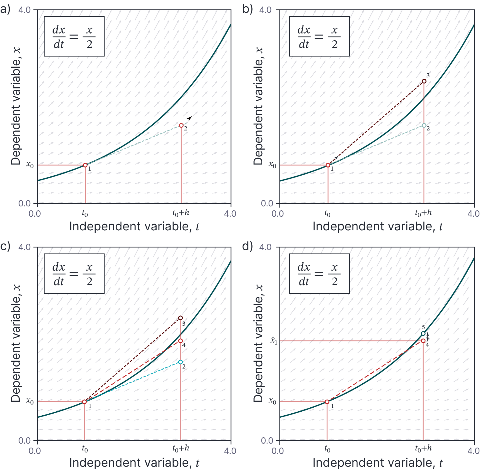
Figure 4. Heun’s method. a) The current solution is projected forward from the initial point (point 1) based on the gradient at this initial point, which takes us to point 2. b) We then measure the gradient at point 2 and project forward again from the initial point (point 1) using this new gradient to reach point 3. c) We average together the two predictions (points 2 and 3) to yield a better estimate (point 4). d) This is the final estimate; notice that the deviation from the true value (point 5) is less than for the Euler method with the same step size.
Comparison of Euler and Heun’s method
Heun’s method requires roughly twice the amount of computation of Euler’s method, but yields more accurate results. Figure 5 shows how the error accrues for the ODE $dx/dt=x/2$ as a function of the step-size $h$. The error for Heun’s method decreases quadratically when the step size is decreased whereas the error for the Euler method only decreases linearly; the minor price of doubling the computation is clearly worth paying.
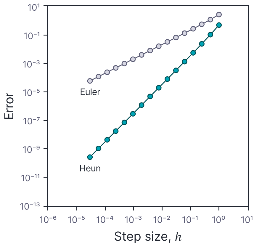
Figure 5. Comparison of Euler and Heun’s methods. Accumulated error over the range [0,4] for the ODE $dx/dt = x/2$ using Euler method (see figure 3b) and Heun’s method as a function of the step size, $h$. For the Euler method the error is $\mathcal{O}[h]$ (i.e., linear with slope one on this log-log plot). For Heun’s method, the error is $\mathcal{O}[h^2]$ (i.e. linear with slope two on this log-log plot). Heun’s method is more costly to implement, but gives much smaller errors for small values of $h$.
Terminology
The previous section contained an informal discussion of two methods to find numerical solutions to ODEs. Now that the basic ideas are in place, we define some terminology relating to numerical methods.
Local vs. global error: At each step, the numerical approximation adds a local truncation error. In contrast, the global error is the total accrued error along multiple steps of the numerical solution.
It is important to note that the global error is not just the sum of the local errors; as we saw in figure 3 the first local error causes the path of the numerical solution $\textrm{x}[t+h]$ to deviate from the true solution, so the gradient $\textrm{f}[x[t+h]]$ at the next step will be wrong. Usually, we can expect the global error to be larger than the sum of the local errors.
Convergence: A numerical method is deemed convergent if the global error decreases to zero as the step size $h$ becomes infinitesimal.
Order of a numerical method: A numerical method is convergent of order $m$ if the global error over the interval of interest decreases as $\mathcal{O}[h^{m}]$. Figure 5 provided evidence that the Euler method is convergent of order one and that Heun’s method is convergent of order two.
Explicit vs. implicit methods: An explicit method only uses the point $\textrm{x}[t]$ that we already know. For example, Heun’s method is explicit:
\begin{equation}
\textrm{x}[t+h] = \textrm{x}[t] + \frac{h}{2}\Bigl( \textrm{f} \bigl[\textrm{x}[t],t\bigr]+
\textrm{f}\Bigl[\textrm{x}[t]+\textrm{f}\bigl[\textrm{x}[t],t\bigr]h,t+h\Bigr]\Bigr),
\tag{8}
\end{equation}
since there are only terms in $\textrm{x}[t]$ on the right-hand side. In contrast, the original trapezoidal update that it approximates is implicit:
\begin{equation}
\textrm{x}[t+h] = \textrm{x}[t] +
\frac{h}{2}\Bigl( \textrm{f} \bigl[\textrm{x}[t],t\bigr]+\textrm{f}\bigl[\textrm{x}[t+h],t+h\bigr]\Bigr),
\tag{9}
\end{equation}
since it uses the term $\textrm{x}[t+h]$. To perform this update, we need to find the value of $\textrm{x}[t+h]$ that makes this equation true. In practice, we could do this by re-arranging the equation as:
\begin{equation}
\textrm{x}[t+h] – \textrm{x}[t] – \frac{h}{2}\Bigl( \textrm{f} \bigl[\textrm{x}[t],t\bigr]+\textrm{f}\bigl[\textrm{x}[t+h],t+h\bigr]\Bigr) = 0,
\tag{10}
\end{equation}
and finding the root for the unknown value $\textrm{x}[t+h]$ using the Newton-Raphson method. This would require much more computation than the explicit formulation of Heun’s method.
One-step vs. multi-step methods: An explicit one-step method has the form:
\begin{equation}
\textrm{x}[t+h] = \textrm{x}[t]+ h \cdot \mbox{g}\bigl[\textrm{x}[t], t\bigr],
\tag{11}
\end{equation}
where $\mbox{g}[\bullet, \bullet]$ is some function of the current estimated position $\textrm{x}[t]$ and time $t$. Both the Euler method and Heun’s method are one-step methods.
In contrast, multi-step methods can also use previous estimates $\textrm{x}[t-h], \textrm{x}[t-2h], \ldots$ from the sequence. For example, a two-step method might have the form:
\begin{equation}
\textrm{x}[t+h] = \textrm{x}[t]+ h \cdot \mbox{g}\bigl[\textrm{x}[t], \textrm{x}[t-h],t\bigr],
\tag{12}
\end{equation}
Adaptive methods: The methods that we have discussed so far use a fixed time-step $h$. In contrast adaptive methods vary the time step as the numerical method progresses. Usually, they have the goal of ensuring that the local truncation error lies within some bound. One approach is to use two methods of different order; the higher-order method can be used to estimate the error due to the lower-order method. If this error is too large, the step size can be decreased (to improve accuracy), and if it is small, the step size can be increased (to improve computational efficiency).
Taylor’s method
We arrived at the Euler method and Heun’s method in an ad-hoc manner by appealing to the Euler and trapezoidal methods for integrating standard functions. Taylor’s method allows us to derive numerical schemes like these in a more principled manner.
Consider a one-step method which has the form:
\begin{equation}\label{eq:ode4_taylor}
\textrm{x}[t+h] \approx \textrm{x}[t]+ h \cdot \mbox{g}\bigl[\textrm{x}[t], t\bigr] ,
\tag{13}
\end{equation}
where $\mbox{g}[\bullet, \bullet]$ is some function of the current position $\textrm{x}[t]$ and time $t$. Consider taking a Taylor expansion of the left hand side of this equation:
\begin{equation}
\textrm{x}[t+h] = \textrm{x}[t] + h \frac{d\textrm{x}[t]}{dt} + \frac{h^2}{2!}\frac{d^2\textrm{x}[t]}{dt^2}+\ldots
\tag{14}
\end{equation}
It follows that we can derive an order $m$ method by choosing $\mbox{g}\bigl[\textrm{x}[t], t\bigr]$ such that $\textrm{x}[t]+ h \cdot \mbox{g}\bigl[\textrm{x}[t], t\bigr]$ matches the first $m$ terms of this expansion.
First-order: For example a first-order method can be derived by setting:
\begin{equation}
\mbox{g}\bigl[\textrm{x}[t], t\bigr] = \frac{d\textrm{x}[t]}{dt},
\tag{15}
\end{equation}
which, when we substitute into equation 13, gives:
\begin{eqnarray}
\textrm{x}[t+h] &\approx & \textrm{x}[t]+ h \frac{d\textrm{x}[t]}{dt} \nonumber \\
&=& \textrm{x}[t]+ h \cdot \textrm{f}\bigl[x[t],t\bigr],
\tag{16}
\end{eqnarray}
where we have substituted the right-hand side of the original ODE $d\textrm{x}[t]/dt = \textrm{f}\bigl[x[t],t\bigr]$ into the second line of the equation. This is the Euler method that we presented before. However, this time we have derived it in a more principled manner.
Second-order: Similarly, a second-order method can be derived by setting:
\begin{equation}
\mbox{g}\bigl[\textrm{x}[t], t\bigr] = \frac{d\textrm{x}[t]}{dt} + \frac{h^2}{2!}\frac{d^2\textrm{x}[t]}{dt^2},
\tag{17}
\end{equation}
which gives the update:
\begin{eqnarray}
\textrm{x}[t+h] & \approx & \textrm{x}[t]+ h\frac{d\textrm{x}[t]}{dt} + \frac{h^2}{2!}\frac{d^2\textrm{x}[t]}{dt^2}\nonumber \\
&=& \textrm{x}[t]+ h \textrm{f}\bigl[x[t],t\bigr] + \frac{h^2}{2!} \frac{d\textrm{f}\bigl[x[t],t\bigr] }{dt}.
\tag{18}
\end{eqnarray}
We can further simplify this expression by substituting in the expression for the total derivative:
\begin{eqnarray}\label{eq:ode4_taylor_total}
\textrm{x}[t+h]
&\approx & \textrm{x}[t]+ h \textrm{f}\bigl[x[t],t\bigr] + \frac{h^2}{2!} \left(\frac{\partial \textrm{f}\bigl[x[t],t\bigr] }{\partial x}\frac{\partial\textrm{x}[t]}{dt} + \frac{\partial \textrm{f}\bigl[x[t],t\bigr] }{\partial t}\right)\nonumber \\
&=& \textrm{x}[t]+ h \textrm{f}\bigl[x[t],t\bigr] + \frac{h^2}{2!} \left(\frac{\partial \textrm{f}\bigl[x[t],t\bigr] }{\partial x}\textrm{f}\bigl[x[t],t\bigr]+ \frac{\partial \textrm{f}\bigl[x[t],t\bigr] }{\partial t}\right).\
\tag{19}
\end{eqnarray}
where we have again substituted in the original definition of the ODE in the second line. This is a valid second-order method and the same technique can be extended to derive higher-order methods. However, this approach introduces the complication of computing derivatives of the original ODE function $\textrm{f}\bigl[x[t],t\bigr]$ with respect to $x$ and $t$. In practice, this means it isn’t used very much, since (as we shall see in the next section) it’s possible to derive higher-order methods that don’t require these derivatives but which have similar properties.
Derivation of Heun’s method: As an aside, we note that Heun’s method can be derived from a further approximation of this second-order formula. We start with:
\begin{eqnarray}\label{eq:ode4_heun_derivation}
\textrm{x}[t+h]
&\approx& \textrm{x}[t]\!+\! h \textrm{f}\bigl[x[t],t\bigr] \!+\! \frac{h^2}{2!} \left(\!\frac{\partial \textrm{f}\bigl[x[t],t\bigr] }{\partial x}\textrm{f}\bigl[x[t],t\bigr]\!+\! \frac{\partial \textrm{f}\bigl[x[t],t\bigr] }{\partial t}\!\right)\tag{20}\\
&=& \textrm{x}[t]\!+\! \frac{h}{2} \textrm{f}\bigl[x[t],t\bigr] \!+\! \frac{h}{2} \left(\!\textrm{f}\bigl[x[t],t\bigr] \!+\! h\textrm{f}\bigl[x[t],t\bigr]\frac{\partial \textrm{f}\bigl[x[t],t\bigr] }{\partial x}\!+\! h\frac{\partial \textrm{f}\bigl[x[t],t\bigr] }{\partial t}\!\right),
\end{eqnarray}
where we have simply re-arranged terms between the two lines. Now we note that the term in the brackets is a truncated Taylor multivariate expansion:
\begin{equation}
\textrm{f}\Bigl[\textrm{x}[t]+h\textrm{f}\bigl[\textrm{x}[t], t\bigr], t+h\Bigr] \approx \textrm{f}\bigl[\textrm{x}[t], t\bigr]+\color{red}h\textrm{f}\bigl[\textrm{x}[t], t\bigr]\frac{\partial \textrm{f}\bigl[\textrm{x}[t], t\bigr]}{\partial x}\color{black}+\color{blue}h\frac{\partial \textrm{f}\bigl[\textrm{x}[t], t\bigr] }{\partial t}\color{black},
\tag{21}
\end{equation}
where the term in red is the change that results from evaluating $\textrm{f}[\bullet,\bullet]$ at position $\textrm{x}[t]+h\textrm{f}\bigl[\textrm{x}[t], t\bigr]$ rather than $\textrm{x}[t]$. Similarly, the term in blue is the change that results from evaluating $\textrm{f}[\bullet,\bullet]$ at time $t+h$ rather than at time $t$.
Substituting this approximation into equation 20 gives Heun’s method:
\begin{eqnarray}
\textrm{x}[t+h] &\approx& \textrm{x}[t] + \frac{h}{2}\textrm{f} \bigl[\textrm{x}[t],t\bigr]+ \frac{h}{2} \textrm{f}\Bigl[\textrm{x}[t]+\textrm{f}\bigl[\textrm{x}[t],t\bigr]h,t+h\Bigr] \nonumber \\
&\approx& \textrm{x}[t] + \frac{h}{2}\Bigl( \textrm{f} \bigl[\textrm{x}[t],t\bigr]+
\textrm{f}\Bigl[\textrm{x}[t]+\textrm{f}\bigl[\textrm{x}[t],t\bigr]h,t+h\Bigr]\Bigr).
\tag{22}
\end{eqnarray}
This gives Heun’s method (which was originally proposed in an ad-hoc manner) some much-needed theoretical justification.
Runge-Kutte methods
Taylor’s method began with an abstract update:
\begin{equation}\label{eq:ode4_rk_setup}
\textrm{x}[t+h] \approx \textrm{x}[t]+ h \cdot \mbox{g}\bigl[\textrm{x}[t], t\bigr] ,
\tag{23}
\end{equation}
and then chose the function $\mbox{g}\bigl[\textrm{x}[t], t\bigr]$ to match the Taylor expansion of the left-hand side up to a given order. Runge-Kutte methods start from the premise that the choice of $\mbox{g}\bigl[\textrm{x}[t], t\bigr]$ is not unique. We can get different expressions that also match the Taylor expansion up to a given order by evaluating the gradient at intermediate points.
Second-order Runge-Kutte
For example, consider an update that fits the template:
\begin{equation}\label{eq:ode4_rk_orig_update}
\textrm{x}[t+h] \approx \textrm{x}[t]+ \omega_1 h \cdot \color{red}\textrm{f} \bigl[\textrm{x}[t],t\bigr] \color{black}+ \omega_2 h\cdot \color{blue}\textrm{f}
\left[x[t]+h\beta \textrm{f} \bigl[\textrm{x}[t],t\bigr],t+\frac{h}{2}\right]\color{black},
\tag{24}
\end{equation}
where $\omega_1, \omega_2,$ and $\beta$ are unknown constants. This expression combines two terms with weights $\omega_1$ and $\omega_2$, respectively. The term in red uses the gradient at the current time. The term in blue makes a guess as to what the gradient will be at time $t+h/2$ (halfway through the integral).
The first-order multivariate Taylor expansion of the term in blue is given by:
\begin{equation}
\color{blue}\textrm{f}
\left[x[t]+h\beta \textrm{f} \bigl[\textrm{x}[t],t\bigr],t+\frac{h}{2}\right] \approx \textrm{f} \bigl[\textrm{x}[t],t\bigr] + h\beta \textrm{f} \bigl[\textrm{x}[t],t\bigr] \frac{\partial \textrm{f} \bigl[\textrm{x}[t],t\bigr]}{\partial x} + \frac{h}{2}\frac{\partial\textrm{f} \bigl[\textrm{x}[t],t\bigr]}{\partial t}
\tag{25}
\end{equation}
which gives the expression:
\begin{eqnarray}\label{eq:ode4_modified_rk}
\textrm{x}[t\!+\!h] \!&\approx&\! \textrm{x}[t]\!+\! \omega_1 h \color{red}\textrm{f} \bigl[\!\!\:\textrm{x}[t],t\bigr] \color{black}\!+\! \omega_2 h \color{blue}\left(\!\textrm{f} \bigl[\!\!\:\textrm{x}[t],t\bigr] \!+\! h\beta \textrm{f} \bigl[\!\!\:\textrm{x}[t],t\bigr] \frac{\partial \textrm{f} \bigl[\!\!\:\textrm{x}[t],t\bigr]}{\partial x} \!+\! \frac{h}{2}\frac{\partial\textrm{f} \bigl[\!\!\:\textrm{x}[t],t\bigr]}{\partial t}\!\right)\color{black}\nonumber \\
\!&=&\! \textrm{x}[t]\!+\! (\omega_1+\omega_2) h \textrm{f} \bigl[\!\!\:\textrm{x}[t],t\bigr] \!+\! \omega_2 h^2 \left( \beta \frac{\partial \textrm{f} \bigl[\textrm{x}[t],t\bigr]}{\partial x}\textrm{f} \bigl[\textrm{x}[t],t\bigr] \!+\! \frac{1}{2}\frac{\partial\textrm{f} \bigl[\textrm{x}[t],t\bigr]}{\partial t}\right).
\tag{26}
\end{eqnarray}
We showed in equation 19 that the Taylor expansion of the left-hand side of equation 23 is:
\begin{equation}\label{eq:ode4_rk_taylor_lhs}
\textrm{x}[t+h] \approx \textrm{x}[t]+ h \textrm{f}\bigl[x[t],t\bigr] + \frac{h^2}{2!} \left(\frac{\partial \textrm{f}\bigl[x[t],t\bigr] }{\partial x}\textrm{f}\bigl[x[t],t\bigr]+ \frac{\partial \textrm{f}\bigl[x[t],t\bigr] }{\partial t}\right).
\tag{27}
\end{equation}
Now we’d like to choose $\omega_1,\omega_2$, and $\beta$ so that the update in equation 26 matches the Taylor expansion in equation 27; this will guarantee that the method is correct up to second-order terms. Matching the three terms between the two equations, we see that:
\begin{eqnarray}
\omega_1+\omega2 &=& 1\nonumber \\
\beta\omega_2 &=& \frac{1}{2}\nonumber \\
\omega_2 &=& 1,
\tag{28}
\end{eqnarray}
which we can solve to find that $\omega_1=0, \omega_2=1, \beta=1/2$.
Substituting these values into our update (equation 24) gives the modified Euler update
\begin{equation}
\textrm{x}[t+h] \approx \textrm{x}[t]+ h \cdot \textrm{f}
\left[x[t]+\frac{h}{2} \textrm{f} \bigl[\textrm{x}[t],t\bigr],t+\frac{h}{2}\right].
\tag{29}
\end{equation}
This is easy to interpret. We propagate to halfway across the interval $(x[t]+\frac{h}{2} \textrm{f}[\textrm{x}[t],t]$) using the current gradient. Then we measure the gradient at this point and use this at the start of the interval to propagate the full way across (see figure 6).
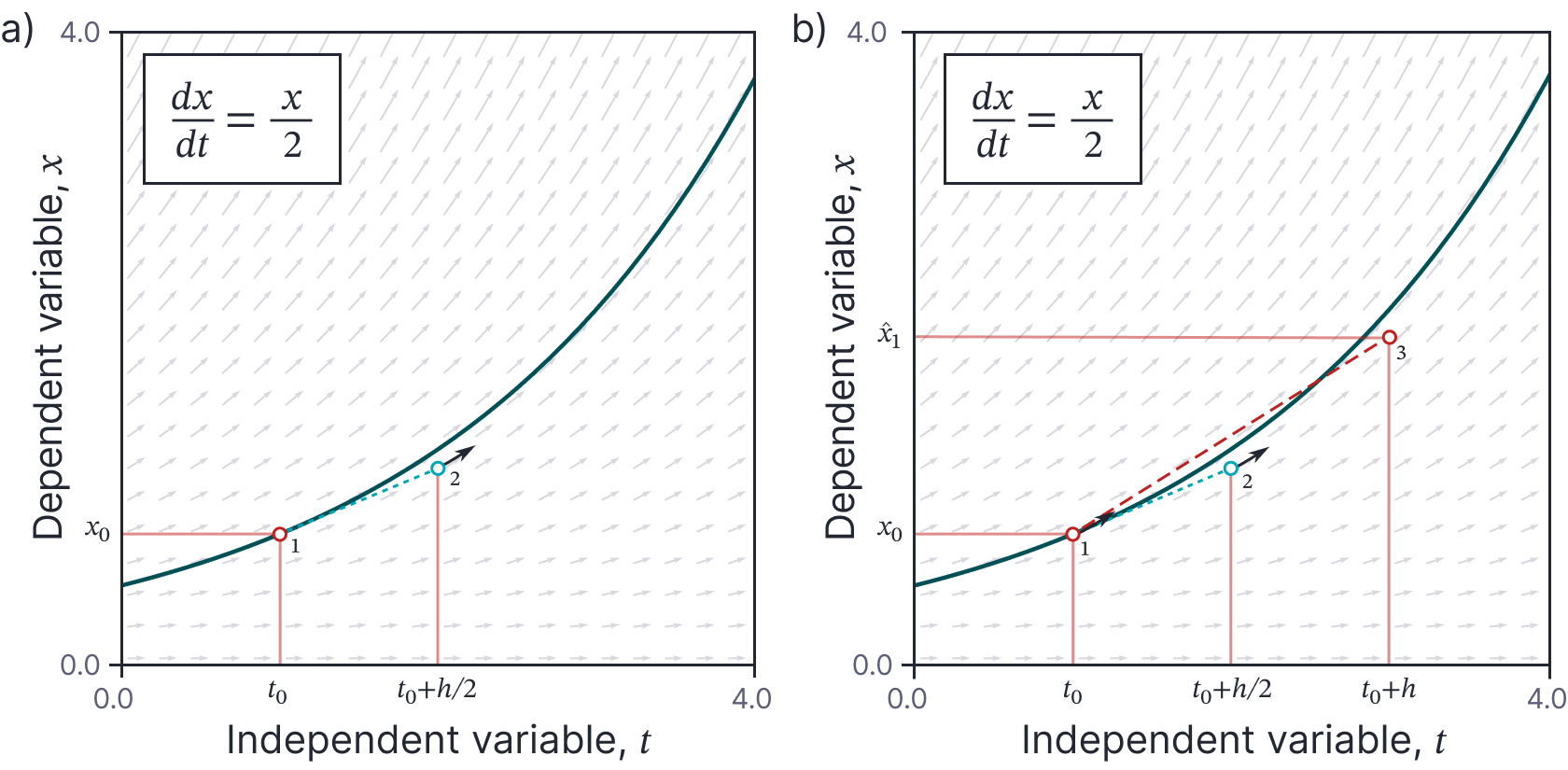
Figure 6. Improved Euler method. a) We start at point 1 and use the gradient to propagate to halfway across the interval (point 2). We measure the gradient at point 2. b) We use this new gradient to propagate from the original point (point 1) across the whole interval. This yields point 3.
Note that we have now presented three order-two methods (Heun’s method, Taylor’s method and the improved Euler method). In general, these will behave slightly differently, but we can expect the errors to scale in the same way with changes in the step size $h$. However, for special case of the example ODE $dx/dt = x/2$, these methods all yield exactly the same results. We leave it as an exercise for the reader to derive explicit updates for all three methods and show that they are the same.
Fourth-order Runge-Kutte
The same approach can be used to derive higher-order numerical methods. As before, we define a template with some unknown parameters, and then select those parameters so that they match the terms in the higher order Taylor expansion.
For example, consider defining the template:
\begin{equation}\label{eq:ode4_runge_kutte_4}
\textrm{x}[t+h] \approx \textrm{x}[t]+ h \cdot \bigl(\omega_1 f_{1}+\omega_2 f_{2}+\omega_3 f_{3}+\omega_4 f_{4}\bigr),
\tag{30}
\end{equation}
where $\omega_{1},\omega_{2},\omega_3,$ and $\omega_4$ are unknown parameters and:
\begin{eqnarray}\label{eq:ode4_runge_kutte4b}
f_{1} &=& \textrm{f}\bigl[x[t],t\bigr]\nonumber \\
f_{2} &=& \textrm{f}\left[x[t]+\frac{1}{2}f_{1}h,t+\frac{1}{2}h\right]\nonumber \\
f_{3} &=& \textrm{f}\left[x[t]+\frac{1}{2}f_{2}h,t+\frac{1}{2}h\right]\nonumber \\
f_{4} &=& \textrm{f}\bigl[x[t]+f_{3}h,t+h\bigr].
\tag{31}
\end{eqnarray}
This template has the following interpretation (figure 7): the first of equations 31 measures the gradient $f_{1}= \textrm{f}\bigl[x[t],t\bigr]$ at the initial point. The second equation propagates from the initial point to halfway across the interval to $t+h/2$ using the gradient $f_{1}$ and measures a new gradient $f_{2}$ at this point. The third equation propagates from the initial point to halfway across the interval using the gradient $f_{2}$ and measures a new gradient $f_3$. The final equation propagates all the way across the interval using the gradient $f_{3}$ and measures a new gradient $f_{4}$ The final result (equation 30) propagates across the whole interval using a weighted sum of these four gradients.
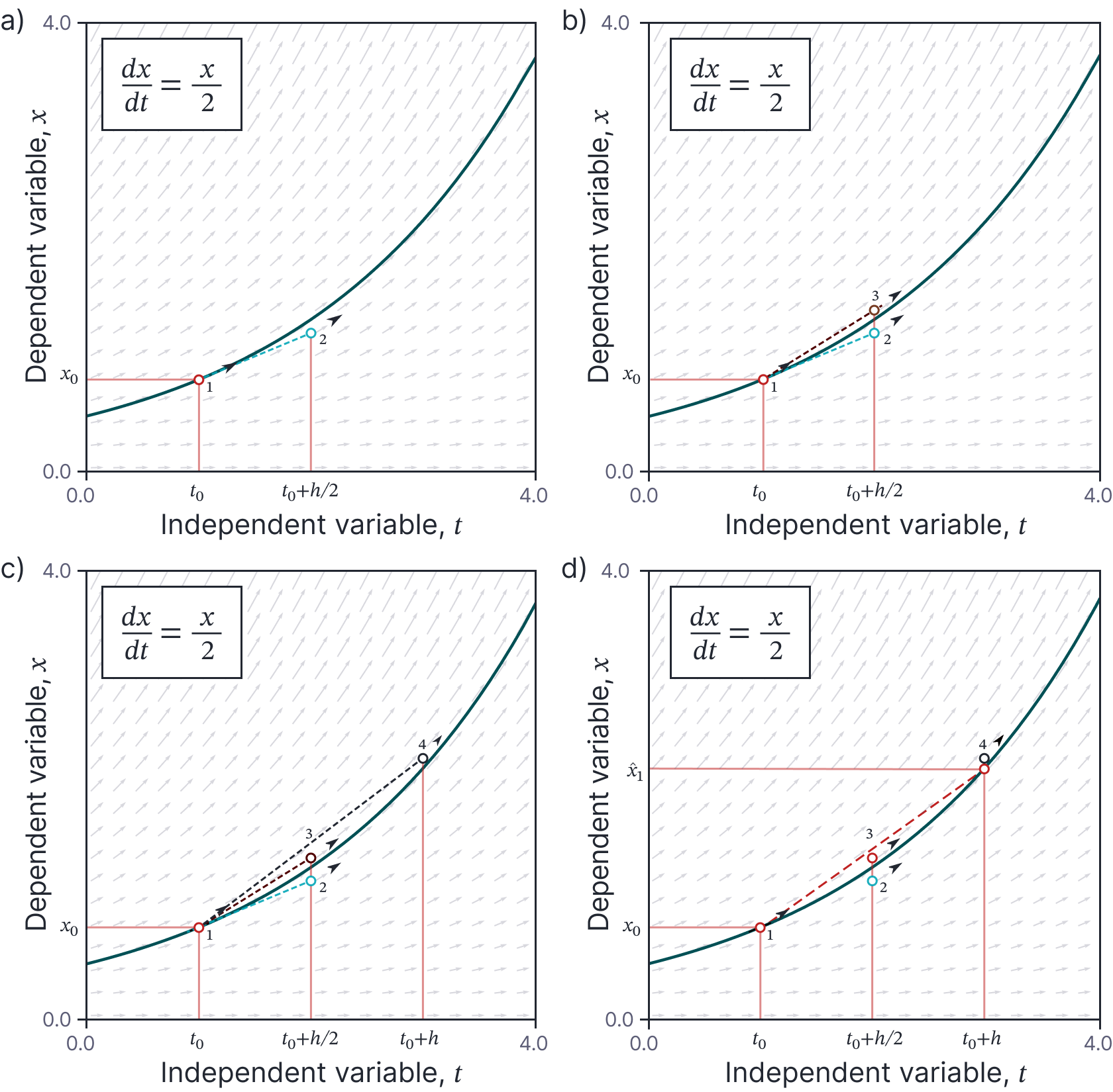
Figure 7. Fourth-order Runge-Kutta method. a) We use the gradient at point 1 to propagate halfway across the interval to point 2. b) We use the gradient from point 2 to propagate halfway across the interval from point 1 to point 3. c) We use the gradient from point 3 to propagate from point 1 to point 4. d) Finally we propagate all the way across the interval using a weighted combination of the gradients at points 1,2,3, and 4.
We find the unknown values $\omega_{1},\omega_{2},\omega_3,$ and $\omega_4$ in exactly the same way as for the second-order case. We expand the left-hand side of equation 30 in a Taylor series, keeping all terms up to fourth order. We then manipulate the right-hand side until it has equivalent terms, and choose the unknown values so the two sides match. The result is the update:
\begin{equation}\label{eq:ode4_runge_kutte_4_known}
\textrm{x}[t+h] \approx \textrm{x}[t]+h\left(\frac{1}{6} f_{1}+\frac{1}{3} f_{2}+\frac{1}{3} f_{3}+\frac{1}{6} f_{4}\right).
\tag{32}
\end{equation}
This method requires obviously requires roughly double the computation relative to the second-order methods. However, the approximation is considerably more accurate; figure 8 compares the five methods that we have seen so far. As expected the accuracy of the fourth-order Runge-Kutte method scales with $h^{4}$. This is often the method of choice for numerical solutions of ODEs.
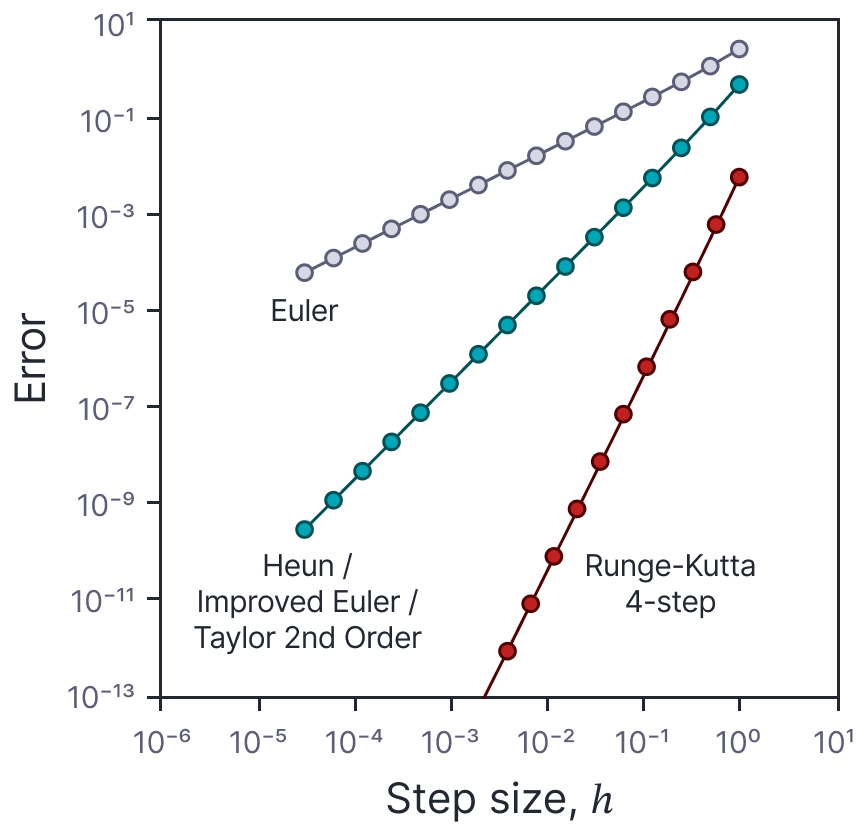
Figure 8. Comparison of numerical solution methods. Accumulated error over the range [0,4] for the ODE $dx/dt = x/2$ as a function of step size for the Euler method (see figure 3b), the Heun, improved Euler, and Taylor second-order methods (which give the same updates for this ODE), and the Runge-Kutte fourth-order method. For the Euler method the error is $\mathcal{O}[h]$ (i.e., a straight line with slope one on this log-log plot). For the second-order methods, the error is $\mathcal{O}[h^2]$ (i.e., a line with slope two on this log-log plot). For the Runge-Kutte fourth-order method the error if $\mathcal{O}[h^4]$ (i.e., a line with slope four on this log-log plot).
Butcher tables
Many numerical methods for solving ODEs including those discussed in this article have the general form:
\begin{equation}
\textrm{x}[t+h] = \textrm{x}[t] + h \sum_{i=1}^{I} \omega_{i} f_{i},
\tag{33}
\end{equation}
where:
\begin{equation}
f_{i} = \textrm{f}\left[\textrm{x}[i]+ \sum_{j=1}^I \beta_{i,j}f_{j}, t+\gamma_i h\right].
\tag{34}
\end{equation}
Here, the final gradient that we use to propagate across the interval is a weighted sum of $I$ gradients $f_{i}$ where the weights are given by $\{\omega_i\}_1^I$. Each of these gradients is computed by propagating a fraction of $\gamma_i$ across the interval using a weighted sum of the other gradients $f_{i}$ where $\beta_{i,j}$ determine these weights.
We can display such schemes visually using a Butcher table or Butcher tableau. For this general case, the Butcher table would be:
\[
\renewcommand\arraystretch{1.2}
\begin{array}
{c|cccc}
\gamma_1 & \beta_{1,1}& \beta_{1,2}& \dots & \beta_{1,I} \\
\gamma_2 & \beta_{2,1}& \beta_{2,2}& \dots & \beta_{2,I} \\
\vdots & \vdots & \vdots & \ddots & \vdots \\
\gamma_I & \beta_{I,1}& \beta_{I,2}& \dots & \beta_{I,I} \\
\hline
& \omega_1 &\omega_2 &\dots &\omega_{I}
\end{array}.
\]
The Butcher tables for the methods discussed in the blog are as follows:
- Euler’s method:
\[
\renewcommand\arraystretch{1.2}
\begin{array}
{c|c}
0 &0 \\
\hline
& 1 \\
\end{array}
\] - Implicit trapezoidal:
\[
\renewcommand\arraystretch{1.2}
\begin{array}
{c|cc}
0 &0 & 0\\
1 & 0 & 1\\
\hline
& \frac{1}{2}& \frac{1}{2}
\end{array}
\] - Heun’s method:
\[
\renewcommand\arraystretch{1.2}
\begin{array}
{c|cc}
0 &0 & 0\\
1 & 1 & 0 \\
\hline
& \frac{1}{2} &\frac{1}{2}
\end{array}
\] - Improved Euler method:
\[
\renewcommand\arraystretch{1.2}
\begin{array}
{c|cc}
0 &0 & 0\\
\frac{1}{2} & \frac{1}{2} & 0\\
\hline
& 0& 1
\end{array}
\] - Fourth-order Runge-Kutte:
\[
\renewcommand\arraystretch{1.2}
\begin{array}
{c|cccc}
0 & 0 & 0 & 0 & 0\\
\frac{1}{2} & \frac{1}{2} &0 & 0 &0\\
\frac{1}{2} &0 &\frac{1}{2} &0 &0 \\
1& 0& 0& 1 & 0\\
\hline
& \frac{1}{6} &\frac{1}{3} &\frac{1}{3} &\frac{1}{6}
\end{array}
\]
Note that for explicit methods, all of the non-zero entries in the Butcher table are in the lower triangular part of the matrix. The sole implicit method that we discussed has a non-zero entry that is on the diagonal. Note that the second-order Taylor’s method cannot be represented in this form.
ODE solvers for machine learning in practice
This article has described some numerical approaches to solving ODEs. In machine learning, the quantity of interest $\textbf{x}[t]$ usually represents the internal state of a network or the parameters during training. As such, it is usually vector-valued rather than scalar valued in these examples. Fortunately, all of the methods described in this article work with vector-valued variables as well without modification. The computation for each scales linearly with the number of dimensions with the exception of the second-order Taylor’s method that would involve computing the matrix of second derivatives and as such scales quadratically.
In general, we won’t have to worry about the internal details of the ODE solvers. Standard ODE packages typically use more complex adaptive methods that are beyond the scope of this article. If we consider a differential equation:
\begin{equation}
\frac{d \textbf{x}[t]}{dt} = \textbf{f}\bigl[\textbf{x}[t],t\bigr],
\tag{35}
\end{equation}
where we know the initial values $\textbf{x}[t_0]$ at time $t=t_0$ and want to find the value at $\textbf{x}[t_1]$ at time $t=t_1$, we can write the solution:
\begin{equation}
\textbf{x}[t_1] = \textbf{x}[t_0] + \int_{t_0}^{t_1} \textbf{f}\bigl[\textrm{x}[\tau],\tau\bigr]d\tau,
\tag{36}
\end{equation}
as the abstract function
\begin{equation}
\textbf{x}[t] = \textbf{ODESolve}\Bigl[\textbf{f}\bigl[\textbf{x}[t],t\bigr], \textbf{x}[t_0], t_{0}, t_{1}\Bigr].
\tag{37}
\end{equation}
Conclusion
This article has developed a series of numerical methods for evaluating ODEs. These are motivated by matching terms in the Taylor expansion of the original function up to a certain order. Higher-order methods require more computation, but errors decreases much more quickly as the step size decreases. The next article in this series will introduce stochastic differential equations.