
This article is the fifth part of our series on ordinary differential equations (ODEs) and stochastic differential equations (SDEs) in machine learning. Part I provided a brief introduction to ODEs and SDEs and how they are applied in machine learning. Part II introduced ODEs and part III and part IV described closed-form and numerical solutions to ODEs, respectively.
This article provides the foundational knowledge that is needed to understand stochastic differential equations. We have seen that that ODEs are formulae that define how a variable changes deterministically over time and that (together with boundary conditions) they implicitly define a function. Analogously, SDEs are formulae that define how a noisy variable changes randomly over time and that (together with boundary conditions) they implicitly describe a stochastic process.
We introduce stochastic processes, which can be thought of as time-varying probability distributions. We consider the Wiener process (Brownian motion), and we see that this is the solution to a simple SDE. We describe other SDEs including those that underpin geometric Brownian motion (used to model asset prices) and the Ornstein-Uhlenbeck process (which underpins diffusion models).
Stochastic processes
A stochastic process is a random variable indexed by time. For the purposes of this article, we will assume that the domain of the random variable and the time dimension are both continuous. A time series is a realization of a stochastic process; it is a set of actual observed values. We can create a time series from a stochastic process by choosing times $t_{1}, t_{2}, t_{3}\ldots t_{T}$, and drawing a joint sample $x_{t_1}, x_{t_2},\ldots x_{t_T}$ from the distribution $Pr(x_{t_1}, x_{t_2}, \ldots x_{t_T})$ implied by the stochastic process.
A stochastic process is considered stationary if it is unaffected by a time shift $\tau$, so that:
\begin{equation}
Pr(x_{t_1}, x_{t_2}, \ldots x_{t_T}) = Pr(x_{t_1+\tau}, x_{t_2+\tau}, \ldots x_{t_T+\tau})
\tag{1}
\end{equation}
To make these ideas concrete, we’ll consider several examples.
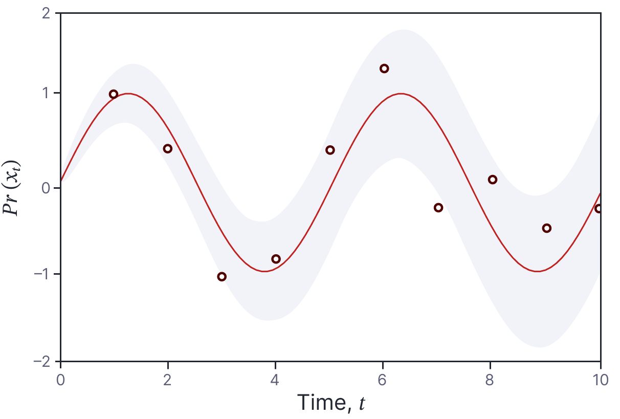
Figure 1. Sinusoidal model. A continuous stochastic process is a random variable indexed by time. This stochastic process (defined in equation 2) is a normal distribution where the mean (blue line) is sinusoidal and the variance (gray region represents $\pm$ two standard deviations) increases as a function of time. If we sample from this continuous stochastic process (red points), we form a time series.
Example 1: sinusoidal model
Consider a normal distribution where the parameters are functions of time:
\begin{equation}\label{eq:ode5_sp_example1}
x_t\sim \mbox{Norm}\Bigl[\sin[\omega t], \sigma^{2} t \Bigr].
\tag{2}
\end{equation}
Here, the mean is a sinusoidal function of $t$ (with angular frequency $\omega$) and the variance increases linearly with time $t$ at a rate of $\sigma^2$ (figure 1). The notation $x_t$ just means that the random variable is a function of time (i.e., it’s short for $x[t]$). We can draw a random sample of the output values at times $t_{1}, t_{2}, t_{3}\ldots t_{T}$ to create a time series of data (red points in figure 1) by simply drawing samples from the independent random variables associated with these times. Note that this process is not stationary; the process explicitly depends on time $t$ and is changed an arbitrary time shift $\tau$.
This stochastic process is easy to understand and to gather time series from but it is not particularly interesting because the random variables at each time are independent. This raises the question of how exactly we might define a stochastic process where the variables at different times have a meaningful joint probability distribution.
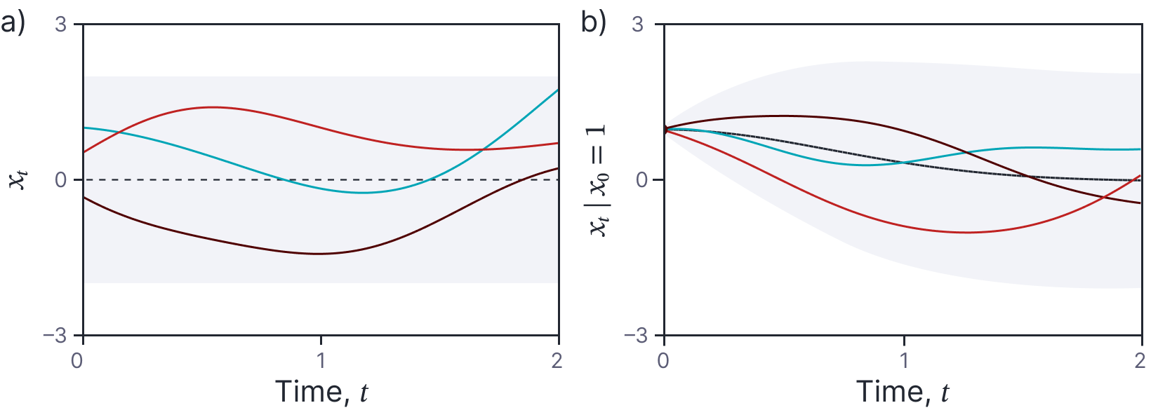
Figure 2. Example Gaussian process. a) The black dashed line represents the mean m[t] and the shaded area represents two standard deviations of the marginal uncertainty (i.e.,, Pr(xt)). The three colored curves are three samples from the Gaussian process. b) If we condition on the point x0 = 1, the resulting samples are constrained to pass through this point.
Example 2: Gaussian processes
One way to specify such a distribution is to define it directly. A Gaussian Process is a collection of random variables, where any finite number of these are jointly normally distributed. It is defined by (i) a mean function $\mbox{m}[t]$ and (ii) a covariance function $\mbox{k}[t,t’]$ that returns the similarity between two points. When we model a function as $\mbox{f}[\mathbf{x}]\sim \mbox{GP}[\mbox{m}[t],\mbox{k}[t,t^\prime]]$ we are saying that:
\begin{eqnarray}
\mathbb{E}\bigl[\mbox{f}[t]\bigr] &=& \mbox{m}[t]\nonumber\\
\mathbb{E}\Bigl[\bigl(\mbox{f}[t]-\mbox{m}[t]\bigr)\bigl(\mbox{f}[t’]-\mbox{m}[t’]\bigr)\Bigr] &=& \mbox{k}[t, t’].
\tag{3}
\end{eqnarray}
The first equation states that the expected value of the function is given by some function $\mbox{m}[t]$ of $t$ and the second equation tells us how to compute the covariance of any two points $t$ and $t’$. As a concrete example, let’s choose:
\begin{eqnarray}
\mbox{m}[t] &=& 0\nonumber\\
\mbox{k}[t, t’]
&=&\mbox{exp}\Bigl[-(t-t’)^{2}\Bigr],
\tag{4}
\end{eqnarray}
so here the expected function values are all zero and the covariance decreases as a function of distance between two points. In other words, points very close to one another will tend to have similar values and those further away will be less similar. Note that this stochastic process is stationary; the mean does not depend on the time $t$ and the covariance only depends on a difference in times $t-t’$. Hence, it is unaffacted by an arbitrary time shift $\tau$.
For any collection of times $t_1, t_2,\ldots t_T$, the random variables $x_{t_1}, x_{t_2},\ldots x_{t_T}$ are normally distributed with mean vector $\boldsymbol\mu$ and a covariance matrix $\boldsymbol\Sigma$:
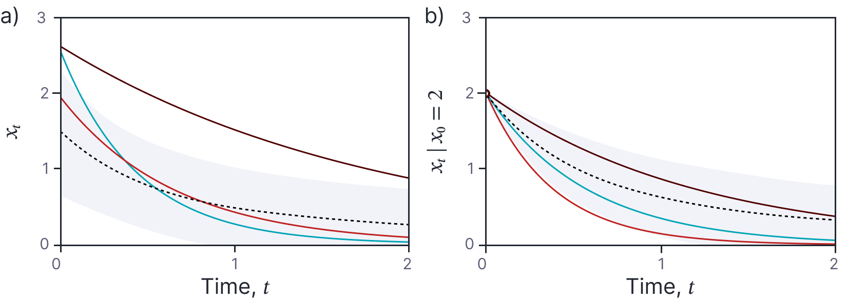
Figure 3. Random exponential decay. a) The black dashed line represents the mean of the stochastic process and the shaded area represents one standard deviation of the marginal uncertainty. The three colored curves are samples from the stochastic process. b) If we condition on the initial point x0 = 2, the resulting samples are constrained to pass through this point and the conditional mean and uncertainty change.
\begin{equation}
\boldsymbol\mu = \begin{bmatrix} m[t_1]\\m[t_2]\\\vdots\\ m[t_T]\end{bmatrix}\quad\quad\quad \boldsymbol\Sigma = \begin{bmatrix}
\mbox{k}[t_1,t_1] & \mbox{k}[t_1, t_2] & \cdots & \mbox{k}[t_1, t_T] \\
\mbox{k}[t_2,t_1] & \mbox{k}[t_2, t_2] & \cdots & \mbox{k}[t_2, t_T] \\
\vdots & \vdots & \ddots &\vdots \\
\mbox{k}[t_T,t_1] & \mbox{k}[t_T, t_2] & \dots & \mbox{k}[t_T, t_T]
\end{bmatrix}.
\tag{5}
\end{equation}
We can sample from this multivariate normal distribution to create time series $x_{t_1}, x_{t_2},\ldots x_{t_T}$ from the stochastic process. Figure 2a shows three time series drawn from this process. We have sampled at regularly spaced intervals and connected these samples so that each result looks like a function (and we shall informally refer to each as such). However, it’s important to remember that we are always visualizing discrete times from an underlying continuous process.
We can also consider conditioning on one or more known points. For example, we can find the distribution $Pr(x_{t_1},x_{t_2},\ldots x_{t_3} | x_{t_0})$ using the standard formula, and draw samples from this conditional distribution. Consider choosing $t_0=0, x_0=1$. Figure 2b depicts the resulting samples, which are still random, but now all pass through this point. We see here the first direct connection with differential equations. The point that we condition on acts like a boundary condition, constraining the behavior of the function at future times. However, unlike in an ODE, this future is not deterministic, but still exhibits randomness.
Example 3: Random exponential decay
For Gaussian processes, we directly specified the joint distribution of the infinite number of random variables associated with all the positions on the continuous timeline. However, for many stochastic processes this is not possible. Hence, it’s common to use an indirect representation. For example, consider the following stochastic process which generates a random decaying function:
\begin{equation}
x_t= u_1 e^{-u_2t},
\tag{6}
\end{equation}
where $u_1\sim \mbox{Uniform}[0,a]$ and $u_2\sim \mbox{Uniform}[0,b]$. Figure 3a shows several time series drawn from this process; each sample is an exponentially decaying function with a random initial height $u_1$ and a random decay speed $u_2$. Once more, we can condition on a known point to get samples that are constrained to pass through this point (figure 3b).
Note that our description of this stochastic process was not explicit; we never defined the joint distribution of $Pr(x_{t_1}, x_{t_2},\ldots, x_{t_T})$. Nonetheless, we might be interested in this joint distribution or other quantities such as the marginal probability distribution $Pr(x_t)$ for each time $t$ or conditional distributions like $Pr(x_{t_2} | x_{t_1}=x)$. Ideally, we would be able to retrieve closed-form expressions for these distributions, but if this isn’t possible, we might at least wish know their moments (mean, covariance etc.).
A simple SDE
Stochastic differential equations are also an indirect way to specify a stochastic process. They are based on the insight that for most real-world quantities, the value at a given time depends on previous values. For example, if the price of some financial asset had a high value at time $t_{1}$, it is likely to have a high value at time $t_{2}$ when the time difference $t_{1}-t_{2}$ is small. A simple way to model this dependence is to define a probability distribution over the change in value of the variable $\Delta x = x_{t_2}-x_{t_1}$ between times $t_{1}$ and $t_{2}$. For example, we might have:
\begin{equation}\label{eq:ode5_delta_change}
Pr(\Delta x) \sim \mbox{Norm}\left[0, \Delta t \right],
\tag{7}
\end{equation}
where the variance is the time interval $\Delta t$; this captures the idea that the value becomes more uncertain with larger time intervals.
Consider how we would generate a time series of observations from this distribution. We choose a value $x_{0}$ at time $t_{0}$. Then we use equation 7 to draw a sample of the change. We use the standard recipe for generating from a normal distribution; we first generate a value $z$ from a standard normal, multiply this by the required standard deviation $\sqrt{\Delta t}$, and finally add the mean (which in this case is zero) to get:
\begin{equation}\label{eq:ode5_delta_sim}
\Delta x = \sqrt{\Delta t} \cdot z,
\tag{8}
\end{equation}
where $z$ is drawn from the standard normal distribution. We add this change to $x_{0}$ to get the new value $x_{1}$ at time $t_{1}=t_{0}+\Delta t$ and repeat this process to generate future values (figure 4a).
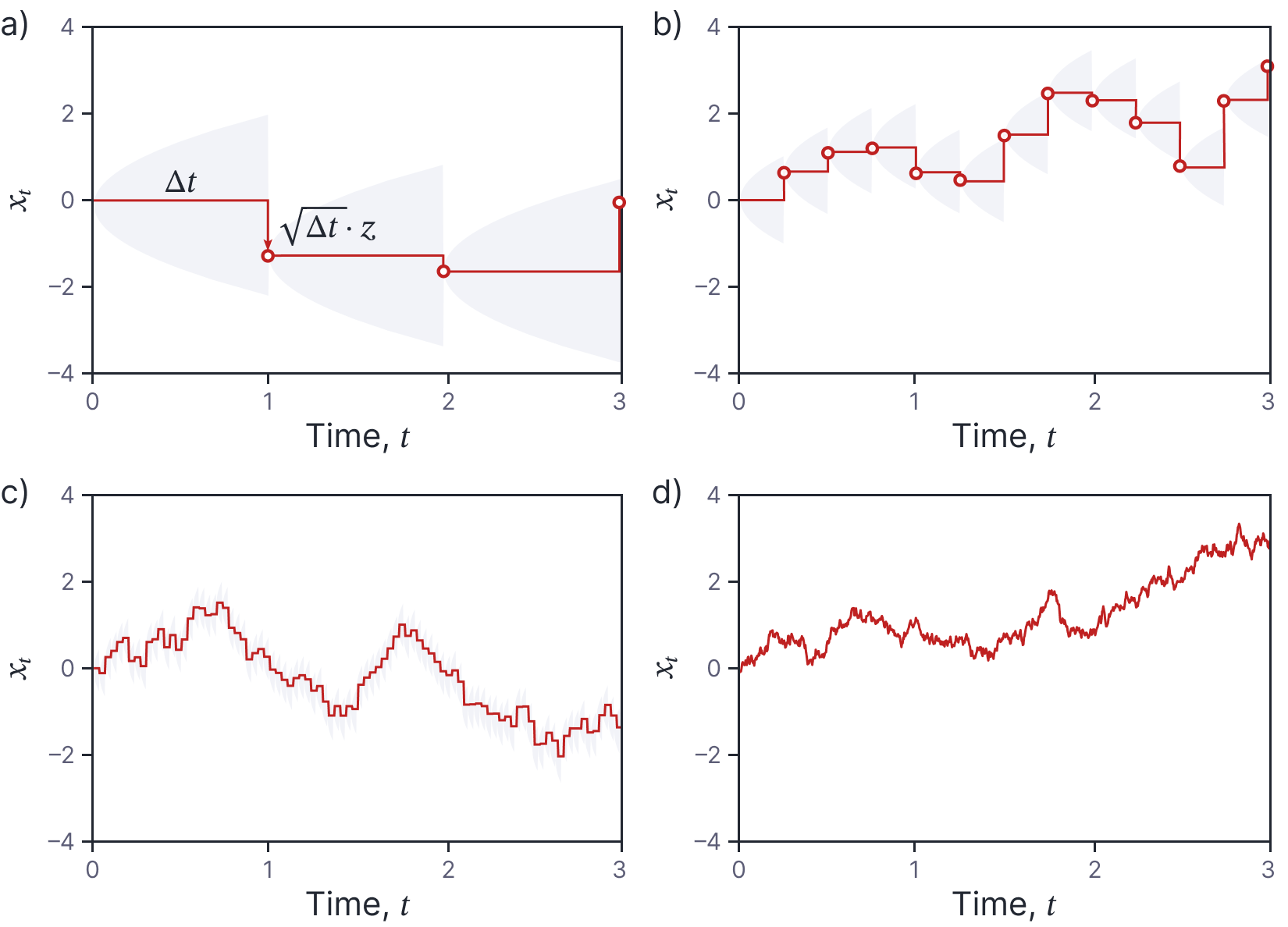
Figure 4. Simple SDE as limit of discrete sampling. The probability Pr(∆x) for a change in x is normal with mean zero and variance that increases proportional to time elapsed. a) If we start with a value of x0 = 0 then the distribution for the next point has mean zero (horizontal orange line) and a variance increasing proportionally with time (gray region represents ±two standard deviations). When we generate a new point (orange circle) by drawing from the distribution, we can think of this as applying
a shock ∆z = √∆tz to the system (vertical orange arrow). The process then continues from the current value. b-c) As we take smaller and smaller time-steps between samples, the resulting curve starts to resemble a noisy real-world quantity such as an asset price. d) In the limit ∆t →0, this becomes a stochastic differential equation.
Taking the limit
As we generate the time series, we can think of the term $\sqrt{\Delta t} \cdot z$ as being a random shock. We’ll modify the notation and represent this shock as $\Delta w = \sqrt{\Delta t} \cdot z$. We now write equation 8 as:
\begin{equation}\label{eq:ode5_delta2}
\Delta x = \Delta w.
\tag{9}
\end{equation}
The related stochastic differential equation (SDE) can be found by considering the limit of this process as the changes in the variable and noise become infinitesimal so that $\Delta x\rightarrow dx$ and $\Delta w = \sqrt{\Delta t} \Delta z \rightarrow dw$ (figure 4b-d):
\begin{equation}\label{eq:ode5_sde_example}
dx = dw.
\tag{10}
\end{equation}
Technically, $dw$ is an an infinitesimal increment of a Wiener process. We will discuss what this means in due course, but for now you can think of it as an infinitesimal contribution of white noise.
Related stochastic process
Equation 10 is arguably the simplest possible SDE; it is roughly equivalent to the ODE $dx/dt=1$. Like all SDEs, it implicitly describes a stochastic process. Like an ordinary differential equation (ODE), this SDE expresses the change in a variable over time given some initial condition (e.g. $x_0=0$). However, the change expressed by the equation is not deterministic, so we get different results each time that we simulate a path.
In practice, we generate a time series by repeatedly running equation 8 for some small time interval $\Delta t$ or equivalently as:
\begin{equation}\label{eq:ode5_wiener_sim}
x_{t} = x_0 + \sum_{s=1}^{t/ \Delta t} \sqrt{\Delta t}\cdot z_s,
\tag{11}
\end{equation}
where $\{z_s\}_{s=1}^{t/\Delta t}$ are draws from a standard normal distribution. This is equivalent to a numerical solution to an ODE, but of course it is different each time due to the stochastic component.
Figure 5 shows several draws from this SDE. The paths generated differ from those produced by an ODE; they are continuous, but nowhere differentiable. We can deduce from these draws that the conditional probability distribution is mean zero and a variance that increases with $t$. It is not (yet) clear how to explicitly define a joint probability distribution $Pr(x_{t_1}, x_{t_2}, x_{t_3}|x_{t_0})$ over points at times $t_1, t_2, t_3$, but this is implicitly specified by the equation; some combinations of $x_{t_1}, x_{t_2}, x_{t_3}$ are definitely more likely than others given that we start at $x_{t_0}$.
Wiener process
The solution to the simple stochastic differential equation $dx = dw$ with boundary condition $x_0=0$ is a stochastic process that is denoted as $W_t$, and referred to as either a Wiener process or Brownian motion. This stochastic process is important as many solutions to more complex SDEs are functions of the Wiener process. In this section, we consider some of its properties, together with some informal arguments as to why these properties hold.
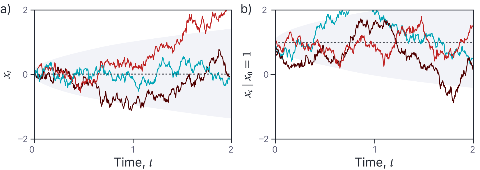
Figure 5. Sample paths from the SDE dx= dw. a) Boundary condition x0 = 0. Dashed black line represents mean of sample and shaded area represents one standard deviation of uncertainty. Three colored lines represents three samples. Technically, these are samples from a “Wiener process.” b) Boundary condition x= 1. Here, the mean of the samples increases accordingly.
Fundamental properties
The Wiener process has the following attributes:
- It starts at zero, so $W_0 = 0$.
- Increments are independent, so $W_v-W_u$ and $W_t-W_s$ are independent if the ranges $[u,v]$ and $[s,t]$ are disjoint.
- Increments in the process are normally distributed so $W_{s+t}-W_{s}\sim \mbox{Norm}[0,t]$.
- With probability one, the function $t\rightarrow W_t$ is continuous.
The first three of these properties can be deduced straightforwardly from equation 11 which we use to simulate the process.
Mean and variance
The first two moments of a Wiener process are given by:
\begin{eqnarray}
\mathbb{E}[W_t] &=& 0 \nonumber \\
\mathbb{E}[W_t^2] &=& t \nonumber \\
\mbox{Var}[W_t] &=& \mathbb{E}[W_t^2] – \mathbb{E}[W_t]^2 = t
\tag{12}
\end{eqnarray}
It is clear that the Wiener process is not stationary since the marginal statistics explicitly depend on the time $t$. These relations can also be deduced from equation 11; the mean is zero because we start at $x_0=0$ and then sum terms, each of which has mean zero. The covariance is $t$ because we divide any interval $t$ into $t/\Delta t$ intervals, each of which has an independent additive contribution of variance $\Delta t$. The variance of the sum of independent variables is the sum of their variances, so we have a final variance of $t/\Delta t \times \Delta t =t$. These properties can be also be derived using the properties of the expectation operator. We leave this as an exercise for the reader.
Covariance
We can also derive the covariance $\textrm{Cov}[W_s, W_t]$ between any two points $s$ and $t$, where $s<t$:
\begin{eqnarray}
\mbox{Cov}[W_s, W_t] &=& \mathbb{E}[(W_s-\mathbb{E}[W_s])(W_t-\mathbb{E}[W_t])]\nonumber\\
&=& \mathbb{E}[W_s W_t] \nonumber \\
&=& \mathbb{E}[W_s(W_t-W_s+W_s)]\nonumber \\
&=& \mathbb{E}[W_s(W_t-W_s)+ W_s^2] \nonumber \\
&=& \mathbb{E}[W_s]\mathbb{E}[W_t-W_s] + E[W_s^2] \nonumber \\
&=& 0 + \mathbb{E}[W_s^2]\nonumber \\
&=& s.
\tag{13}
\end{eqnarray}
where we have used the fact that $\mathbb{E}[W_{s}] = \mathbb{E}[W_{t}] = 0$ between lines one and two and the fact that $\mathbb{E}[W_{s}]$ is zero and is independent from $\mathbb{E}[W_{t}-W_s]$ when $s<t$ between lines five and six. In general $\mbox{Cov}[W_s, W_t]=\min[s,t]$.
Markov property
The future of the Wiener process after time $t_0$ depends only on its current value at time $t_0$ and is independent of values before time $t_0$ so:
\begin{equation}
W_{t_0+t} = W_{t_0} + \bigl(W_{t_0+t}-W_{t_0}\bigr),
\tag{14}
\end{equation}
where the second term is independent of the past due to the independence of increments (fundamental property 2).
Scaling properties
The Wiener process has a number of scaling properties. If we multiply a Wiener process process by minus one (i.e. flip the axes vertically), we get another Wiener process so $(-W_{t})_{t\geq 0}$ is a Wiener process. If we translate a Wiener process in time by a constant $s$ we get another Wiener process so $(W_{t+s}-W_s)_{t\geq 0}$ for fixed $s$ is a Wiener process. If we stretch time (zoom in horizontally) by a factor $c$ and scale the result by $1/\sqrt{c}$ then we get another Wiener process so $W_{ct}/\sqrt{c}$ is a Wiener process for $c>0$. If we invert the time axis but also scale by $t$ then we get another Wiener process so $(t W_{1/t})_{t\geq 0}$ is a Wiener process.
Differentiability
With probability one, the sample paths of a Wiener process are not Lipschitz continuous and are hence non-differentiable at any point. For an informal proof of this, consider trying to compute the derivative as:
\begin{equation}
\frac{dW_t}{dt} = \lim_{h\rightarrow 0} \frac{W_{t+h}-W_{t}}{h}.
\tag{15}
\end{equation}
We know that $W_{t+h}-W_{t}\sim \mbox{Norm}[0, h]$ and so $(W_{t+h}-W_{t})/h\sim \mbox{Norm}[0, 1/h]$ (using the linear transformation property of the Gaussian). It follows that as $h\rightarrow 0$ the variance term explodes and the random variable does not converge. Regardless of the fact that the derivative of a Wiener process does not really exist, it’s common to refer to it as white noise.
Time-changed Brownian motion
Sometimes, we want to describe a Wiener process in some function $\mbox{f}[t]$ instead of in $t$. For example, we might have $\mbox{f}[t]=\exp[t]$, which we write as $W_{\exp[t]}$. This process has moments:
\begin{eqnarray}
\mathbb{E}[W_{\exp[t]}] &=& 0 \nonumber \\
\mathbb{E}[W_{\exp[t]}^2] &=& \exp[t] \nonumber \\
\mbox{Var}[W_t] &=& \mathbb{E}[W_{\exp[t]}^2] – \mathbb{E}[W_{\exp[t]}]^2 = \exp[t].
\tag{16}
\end{eqnarray}
By a similar logic, this process has covariance:
\begin{eqnarray}
\mbox{Cov}[W_{\exp{s}}, W_{\exp{t}}]&=&\min\bigl[\exp[s],\exp[t]\bigr]\nonumber \\
&=& \exp\bigl[\min[s,t]\bigr].
\tag{17}
\end{eqnarray}
Stochastic differential equations
We have introduced the idea of a stochastic process and investigated the very simple stochastic differential equation:
\begin{equation}
dx = dw,
\tag{18}
\end{equation}
with boundary condition $x_0$, which has solution $x_0+ W_{t}$, where $W_{t}$ is a Wiener process. Let’s now extend these ideas to more complex SDEs.
In general a stochastic differential equation implicitly describes a noisy evolving variable $x$ by defining changes $dx$ in that variable in the infinitesimal limit of time. In this article, we will assume that the underlying noise component is normally distributed, so a more general formulation of an SDE has the form:
\begin{equation}\label{eq:ode5_general_sde}
dx = \mbox{m}[x,t] dt + \mbox{s}[x,t] dw,
\tag{19}
\end{equation}
where $x$ is the dependent variable and $t$ is the independent variable (usually representing time). The term $dx$ represents an infinitesimal change in the dependent variable, the term $dt$ represents an infinitesimal change in time, and $dw$ represents an infinitesimal noise shock. The drift term $m[x,t]$ and the diffusion term $s[x,t]$ control the magnitude of the deterministic and stochastic changes to the variable, respectively. If neither the drift term, nor the diffusion term depend explicitly on the time $t$, we say that this is a process with stationary increments. However, as we saw for the Wiener process, this does not necessarily imply that the corresponding random process is stationary. The solution to the SDE is a stochastic process and will typically be some function of the Wiener process $W_{t}$.
Just as for ODEs, we can also consider SDEs in vector quantities $\mathbf{x}$ which have the general form:
\begin{equation}
d\mathbf{x} = {\bf m}[\mathbf{x},t] dt + {\bf S}[\mathbf{x},t] d\mathbf{z},
\tag{20}
\end{equation}
where ${\bf m}[\mathbf{x}, t]$ is a vector valued function and ${\bf S}[\mathbf{x},t]$ is a matrix valued function that mixes the independent noise components in $\mathbf{z}$.
To make these ideas more concrete, let’s now consider two widely-used examples of stochastic differential equations that fit the general formulation in equation 19.
Example 1: Geometric Brownian motion
A common application for SDEs is to model the evolution of asset prices. However, the simple SDE described above doesn’t produce data that resembles observed time series for asset values; it can produce negative values, and it does not capture the tendency of stock values to increase on average over time at an increasing rate (like compound interest in a bank account). Moreover, for real stock values, we expect the noise to be proportional to the value, so that the probability of change of $\pm 5\%$ would be the same whether the stock price was high or low.
This behavior can be captured by the Geometric Brownian motion SDE:
\begin{equation}\label{eq:ode5_sp_geo}
dx = \mu x dt + \sigma x dw,
\tag{21}
\end{equation}
where $\mu$ and $\sigma$ are known parameters. Clearly this is a special case of equation 19. Sample paths from this SDE are illustrated in figure 6. Notably, the paths are always positive if initialized with a positive value, and both the mean of the process and the variance functions increase with the current value $x$. In the context of the Geometric Brownian model, the parameter $\sigma$ that controls the amount of noise is known as the volatility.
The solution to the geometric Brownian model can be expressed in terms of the Wiener process and is (non-obviously):
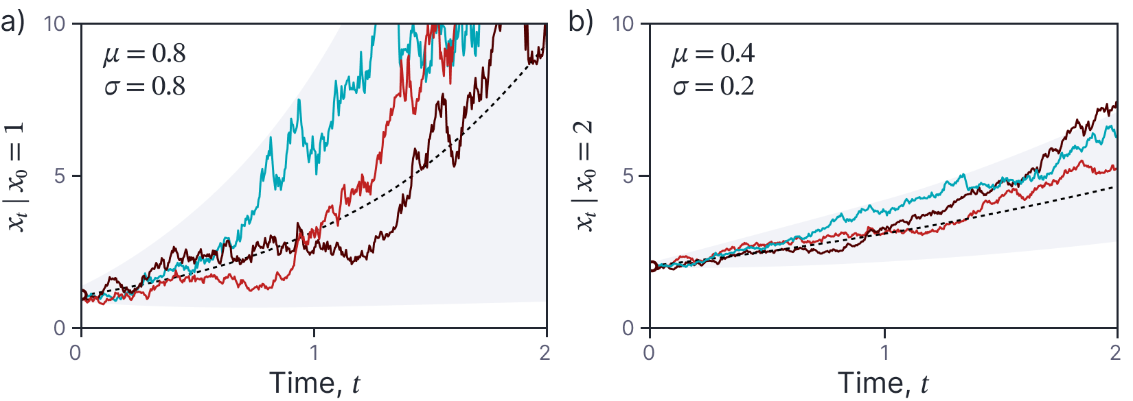
Figure 6. Geometric Brownian motion. a) Three colored curves represent samples generated from equation 1.21 with parameters µ = 0.8,σ = 0.8 and initial condition x0 = 1. Black dashed line represents the mean of the stochastic process and the gray region represents the 95% confidence interval. b) Geometric Brownian motion with parameters µ = 0.4,σ = 0.2 and initial condition x0 = 2. Here the growth is slower and the functions are less noisy than in panel (a).
\begin{equation}
x_{t}= x_{0} \exp\Biggl[\left(\mu – \frac{1}{2}\sigma^2 \right)t + \sigma_{t} W_{t}\Biggr].
\tag{22}
\end{equation}
We will show how to derive this result in the next article in this series.
Example 2: Ornstein-Uhlenbeck process
The Ornstein-Uhlenbeck process has associated SDE:
\begin{equation}
dx = -\gamma x \cdot dt + \sigma \cdot dw,
\tag{23}
\end{equation}
with parameters $\gamma\geq 0$ and $\sigma > 0$. Note that this is very similar to the Geometric Brownian motion model, but the noise is no longer scaled by the current value $x$.
A special case of the Ornstein-Uhlenbeck process is the diffusion model used in machine learning:
\begin{equation}\label{eq:ode5_sp_diffusion}
dx = -\frac{1}{2} \beta x \cdot dt + \sqrt{\beta}\cdot dw,
\tag{24}
\end{equation}
where first term attenuates the data plus any noise added so far, and the second adds more noise. The parameter $\beta\in[0,1]$ determines how quickly the noise is blended. The solution to the equation always converges to a standard normal distribution as $t\rightarrow\infty$. Draws from this SDE are illustrated in figure 7.
The solution to this SDE is (non-obviously):
\begin{equation}
x_{t} = x_0\exp[-\gamma t] + \frac{\sigma}{\sqrt{2\gamma}} W_{1-\exp[-2\gamma t]}.
\tag{25}
\end{equation}
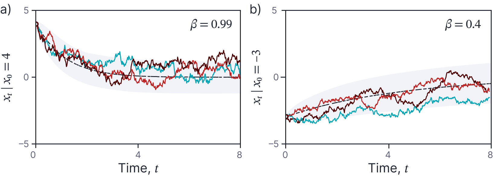
Figure 7. Diffusion SDE. a) Colored lines represent three samples from the diffusion SDE (equation 1.24) with parameter β = 0.99 and initial condition x0 = 4. Black dashed line represents the mean of the process and the gray region represents the 95% confidence region. b) Diffusion process with parameter β = 0.4. The mean and variance of the samples always converges to a standard normal distribution as t→∞.
Note that in this case, we can only express the solution in terms of an integral; we cannot directly describe the solution as a function of the Wiener process.
ODEs vs. SDEs
This article has characterized SDEs as implicit representations of stochastic processes. In this final section, we explicitly compare ODEs and SDEs.
Visualization: An ODE with one dependent variable and one independent variable can be visualized as a vector field (figure 8a). An initial point is propagated by following the direction of this field at every point. Conversely, an SDE with one dependent variable and one independent variable can be visualized as a probabilistic vector field (figure 8b). At each point in the vector field, there is a distribution of possible directions. A point is propagated forward by randomly sampling from these distributions at each position.
Closed-form solutions: The solution to an ODE is a function and we hope to find a closed-form expression for this function. Conversely, the solution to an SDE is a stochastic process. Similarly, we hope to find a closed-form expression for this stochastic process (often a function of a Wiener process). However, sometimes, this is not possible and we settle for closed-form expressions for the moments (mean, variance, etc.) as function of time.
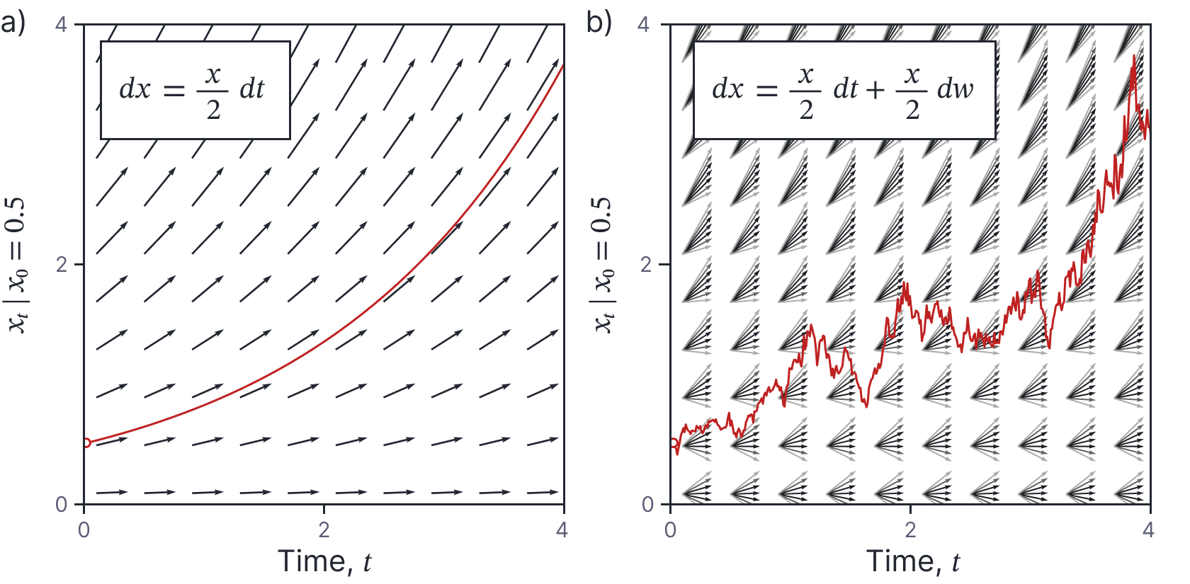
Figure 8. ODEs vs SDEs. a) An ODE can be visualized by a vector field and a function that obeys the ODE will be aligned with this vector field at every point. b) An SDE can be visualized as a probabilistic vector field where there is a distribution of possible vector directions at every position (darker arrows represent higher probability). A function that obeys the SDE will sample from this distribution at each position to determine its next value.
Method of solution: Closed-form solutions to ODEs are found by integration (i.e., using standard calculus). However, SDEs are solved using stochastic calculus. This has different rules from the standard calculus that you are familiar with. For example, the chain rule is different, and the rules for changing variables are not the same. This is a result of Itô’s famous lemma, which we will study this is the next article in this series.
Numerical solutions: When we cannot solve an ODE in closed-form, we can still find a numerical solution by starting at some initial condition and propagating this solution forward; we alternately (i) evaluate the ODE to determine how the function is changing at the current position and (ii) use this information to predict where the solution will be shortly thereafter. We can apply exactly the same approach to SDEs, but now the gradient is stochastic and so the paths are different each time. When a closed-form solution is not available, it is typical to compute many such paths and use the statistics of these to estimate the mean and variance of the stochastic process as a function of time.
Initial conditions: An ODE defines a family of functions. Adding an initial condition $x_0$ determines the particular member of this family. Similarly, an SDE really defines a family of stochastic processes and adding an initial condition $x_0$ determines the particular stochastic process. However, for SDEs we might more generally define the initial conditions as a probability distribution $Pr(x_0)$ (figure 9). Indeed, we can consider a known initial value $x_0$ as a special case where this distribution is a delta function $\delta[x-x_0]$ at $x_0$.
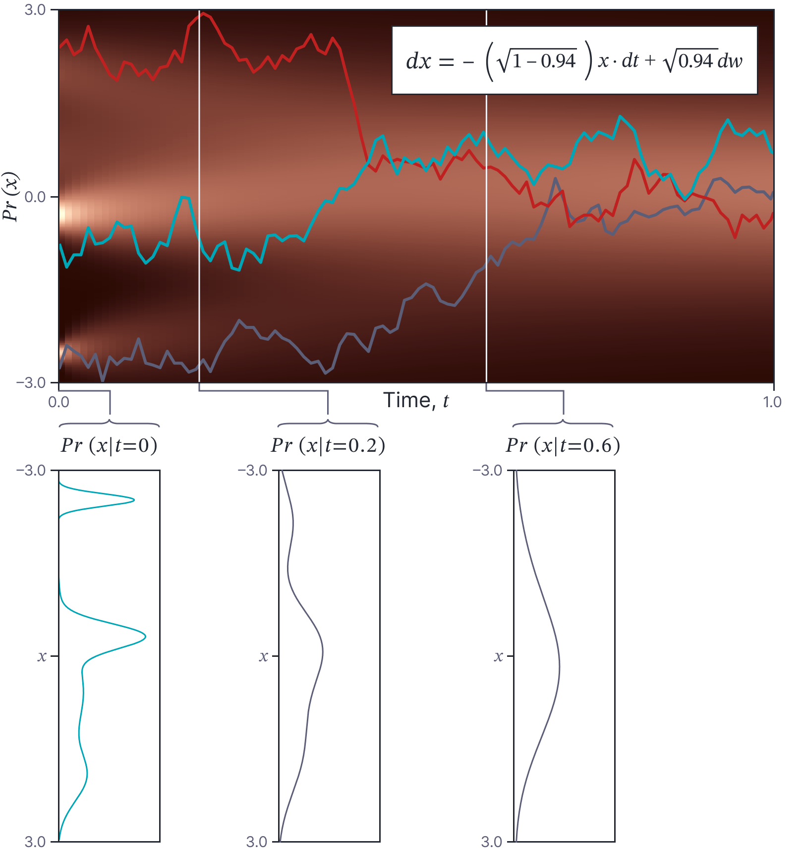
Figure 9. Probability distribution as an initial condition. In this SDE, the initial condition is not a single value but a probability distribution $Pr(x|t=0)$. This probability is represented by the intensity in the left column of the main image. As the SDE evolves (moving right across the image), this probability changes. In this case, the SDE is a diffusion equation and so the probability $Pr(x|t)$ becomes a standard normal distribution as $t\rightarrow \infty$. Three colored paths represent three draws from initial distribution and their subsequent trajectory
Reversing time: It’s possible to define a reverse-time ODE (where we start with the boundary condition $x_T$ at some time $t_T$ and work backwards). In practice, we simply multiply the right-hand side of the ODE by minus one to find the equivalent reverse time ODE. However, this does not work for SDEs; when we multiply the right-hand side of an SDE by minus one, the drift term changes direction, but the diffusion term stays the same; it is is based on a symmetric noise update $dw$ and multiplying this by minus one makes no difference (due to the scaling property under inversion); Consequently, we still add noise whichever direction we move in. Hence, we cannot just propagate solutions back and forth without modification. In part VIII of this series, we will discuss Andersen’s theorem which describes how to reverse the direction of an SDE, so that the marginal distributions remain the same as for the forward process.
Summary
This article introduced stochastic processes using a series of examples. We saw that many stochastic process can only be described implicitly and that stochastic differential equations are such a method of implicit description. We developed the simple SDE $dx=dw$ by considering the limit of an incremental noise process. We defined the solution of this equation to be a Wiener process and described its properties.
We considered more general SDEs and described two concrete examples: geometric Brownian motion (used to represent asset prices) and the SDE associated with the Ornstein-Uhlenbeck process (used in denoising diffusion models). Finally, we compared the properties of ODEs and SDEs.
In the next articles in this series, we will investigate stochastic calculus and use this to find closed-form solutions to some SDEs (part VII). Just as for ODEs an important method is to use a change of variables to convert an intractable SDE to one for which a solution is readily available. To this end, we will derive Itô’s lemma which illuminates how such changes must be made. We will also present Andersen’s theorem which is used to reverse the direction of SDEs and the Fokker-Plank equation which maps an SDE to an PDE that determines the evolution of the probability distribution associated with the SDE.