
This is the eighth in a series of articles concerning the use of ordinary differential equations (ODEs) and stochastic differential equations (SDEs) in machine learning. Part I provided a high-level overview of this area. Part II, part III, and part IV introduced ordinary differential equations and investigated closed-form and numerical solutions, respectively. Part V introduced stochastic differential equations and stochastic processes. Part VI and part VII developed methods to solve stochastic differential equations by direct integration and the use of Itô’s lemma, respectively.
Part VIII of this series (this article) concludes our treatment of SDEs with a discussion of the Fokker-Planck equation and Anderson’s reverse-time SDE theorem. Although an individual path through an SDE is noisy, the evolution of the marginal distribution of this noise is deterministic. The Fokker-Planck equation exploits this insight; it takes a stochastic differential equation and turns it into a partial differential equation for the associated probability distribution.
Reversing time for ordinary differential equations is easy; since the evolution is deterministic, we can simply reverse the sign of the right-hand side ODE and run time backwards. However, for stochastic differential equations this does not work. Whichever way we run the SDE, the noise term increases the uncertainty and so we never get back to the initial conditions. Anderson’s reverse-time SDE theorem shows how to modify the reverse SDE so that its marginal distributions match those of the forward process.
Fokker-Planck equation
The previous articles in this series solved SDEs directly and found closed-form expressions for the underlying stochastic processes. This section takes a different approach. We first convert the stochastic differential equation to a partial differential equation (PDE) where the dependent variable is the probability distribution of possible solutions. Then we solve this PDE to recover the stochastic process.
From SDEs to stochastic processes
Consider a stochastic differential equation of the form:
\begin{equation}
dx = \mbox{m}[x,t] dt + \mbox{s}[x,t] dw,
\tag{1.1}
\end{equation}
where $x$ is the dependent variable, $t$ is the independent variable, $\mbox{m}[x,t]$ is the drift term that governs how $x$ changes deterministically in an infinitesimal time increment $dt$ and $\mbox{s}[x,t]$ is the diffusion term that governs how the infinitesimal noise $dw$ contributes.
Given an initial condition $x_0$ at time $t=0$, we can simulate this equation by approximating $dt$ and $dw$ with finite but small quantities $\Delta t$ and $\Delta w$ and iteratively computing small changes $\Delta x$. Each time we do this, we get a different result due to the noise inherent to the contribution of the diffusion term.
When we solve this SDE, we recover the underlying stochastic process. This is a probability distribution that is indexed by time. Often, we express this in terms of the evolving moments of the marginal distributions. For example, in part VII of this series we considered the Ornstein-Uhlenbeck equation:
\begin{equation}
dx = -\gamma x dt + \sigma dw,
\tag{1.2}
\end{equation}
and showed that its solution was given by:
\begin{equation}
p(x, t) \sim \mbox{Norm}_{x}\left[x_0\exp[-\gamma t], \frac{\sigma^2}{2\gamma}\Bigl(1-\exp[-2\gamma t]\Bigr)\right].
\tag{1.3}
\end{equation}
This closed-form expression for the evolving probability distribution suggests that there might be an underlying deterministic differential equation that governs how the probability distribution changes in each infinitesimal time-period. Since the probability $p(x,t)$ is a function of both $x$ and the time $t$, this will be a partial differential equation (PDE) with dependent variable $p(x,t)$ and independent variables $x$ and $t$ (figure 1.1). Note we are following the convention from physics, we write $p(x,t)$, but this is not a joint distribution in $x$ and $t$; it is the conditional distribution $p(x|t)$ and sums to one for any time $t$, and the interpretation of $t$ in p(x,t)$ is that of a parameter.
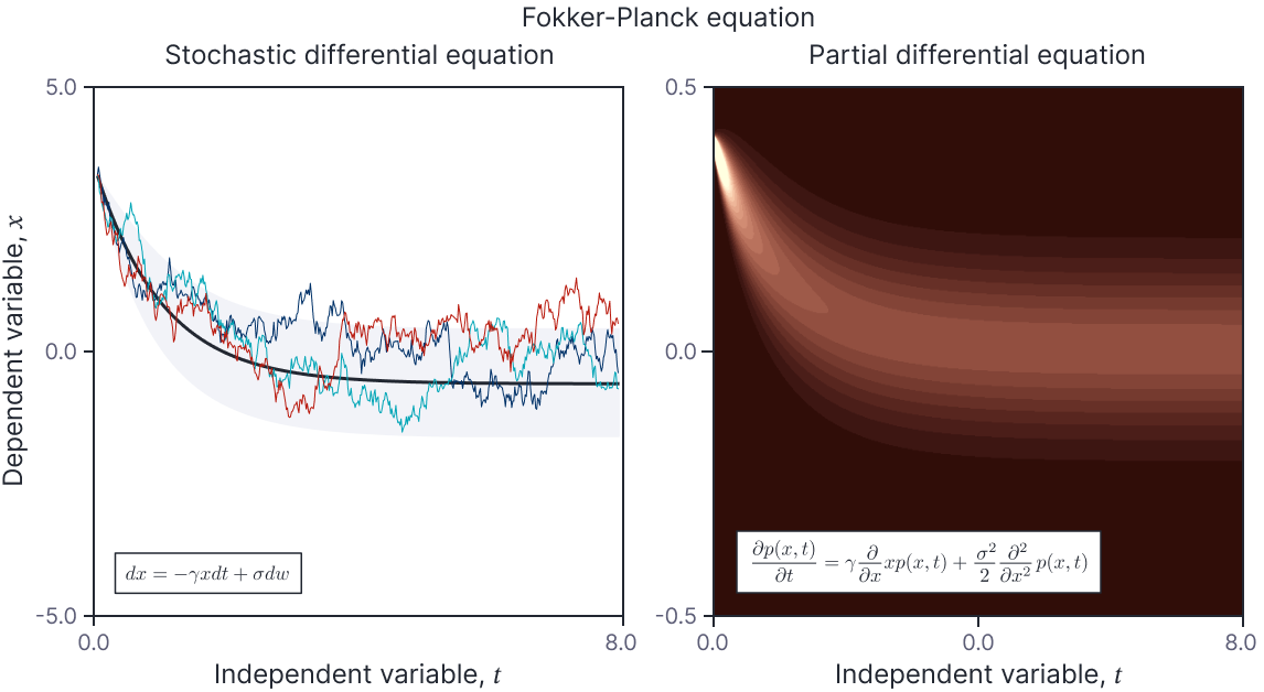
Figure 1.1 Fokker-Planck equation. An SDE (left) considers the stochastic evolution of the dependent variable, and when we solve the SDE, we recover the marginal distributions of the underlying stochastic process (grey regions represent $\pm 2$ standard deviations). The Fokker-Planck equation converts this SDE into a partial differential equation that models the deterministic evolution of the probability distribution over $x$ (right).
A PDE for the probability distribution
The Fokker-Planck equation (also known as the Kolmogorov equation) provides a method to find this partial differential equation. It states that for a stochastic differential equation of the form:
\begin{equation}
dx = \mbox{m}[x,t] dt + \mbox{s}[x,t] dw,
\tag{1.4}
\end{equation}
the probability distribution $p(x,t)$ of the variable $x$ evolves as:
\begin{equation}
\frac{\partial p(x,t)}{\partial t} = -\frac{\partial }{\partial x} \textrm{m}\bigl[x,t]p(x,t)+\frac{1}{2}\frac{\partial^2}{\partial x^2} s[x,t]^2 p(x,t).
\tag{1.5}
\end{equation}
Consider the multivariate SDE:
\begin{equation}
d\mathbf{x} = \mathbf{m}[\mathbf{x},t] dt + \mathbf{S}[\mathbf{x},t] d\mathbf{w},
\tag{1.6}
\end{equation}
in $\mathbf{x}\in\mathbb{R}^{D}$. The equivalent relation is given by:
\begin{align}
\frac{\partial p(\mathbf{x},t)}{\partial t} &= -\sum_{i=1}^{D} \frac{\partial }{\partial x_{i}} \mbox{m}_{i}[\mathbf{x},t] p(\mathbf{x},t) \nonumber\\&\hspace{1cm}+\frac{1}{2}\sum_{i,j=1}^{D} \frac{\partial^2}{\partial x_{i}\partial x_{j}}\Bigl( \mathbf{S}[\mathbf{x},t]\mathbf{S}^T[\mathbf{x},t]\Bigr)_{i,j} p(\mathbf{x},t).\tag{1.7}
\end{align}
Proof of the Fokker-Planck relation
Consider a function $\mbox{f}[x,t]$. Itô’s lemma for a change in variables states that:
\begin{equation}
df = \left(\frac{\partial f}{\partial t} + \frac{\partial f}{\partial x}\mbox{m}[x,t] + \frac{1}{2} \frac{\partial^{2} f}{\partial x^{2}}\mbox{s}[x,t]^{2} \right)dt + \frac{\partial f}{\partial x} \mbox{s}[x,t]dw.
\tag{1.8}
\end{equation}
Taking expectations, we have:
\begin{eqnarray}
\mathbb{E}\bigl[df\bigr]= \Biggl( \mathbb{E}\biggl[\frac{\partial f}{\partial t} \biggr]+\mathbb{E}\biggl[\frac{\partial f}{\partial x}\mbox{m}[x,t]\biggr] +\frac{1}{2}\mathbb{E}\biggl[\frac{\partial^2 f}{\partial x^2} s[x,t]^2 \biggr]\Biggr)dt,
\tag{1.9}
\end{eqnarray}
where the final term has disappeared as $\mathbb{E}[dw]=0$. Dividing both sides by $dt$, we have:
\begin{eqnarray}
\frac{d}{dt}\mathbb{E}\bigl[f\bigr] &=& \mathbb{E}\biggl[\frac{\partial f}{\partial t} \biggr]+\mathbb{E}\biggl[\frac{\partial f}{\partial x}\mbox{m}[x,t]\biggr] +\frac{1}{2}\mathbb{E}\biggl[\frac{\partial^2 f}{\partial x^2} s[x,t]^2 \biggr]
\tag{1.10}
\end{eqnarray}
or writing out the integrals explicitly:
\begin{eqnarray}
\int\frac{d}{dt} p(x,t) \mbox{f}[x,t] dx=\int p(x,t)\frac{\partial \mbox{f}[x,t]}{\partial t}dx &&\tag{1.11}\\
&&\hspace{-8cm}+\int p(x,t)\frac{\partial \mbox{f}[x,t]}{\partial x}\mbox{m}[x,t]dx +\frac{1}{2}\int p(x,t)\frac{\partial^2 \mbox{f}[x,t]}{\partial x^2} s[x,t]^2dx.
\end{eqnarray}
The left hand side can be expanded using the chain rule:
\begin{eqnarray}
\int\frac{d}{dt} p(x,t) \mbox{f}[x,t] dx &=& \int \frac{d p(x,t)}{dt}\mbox{f}[x,t]dx + \int p(x,t)\frac{d \mbox{f}[x,t]}{dt}dx.
\tag{1.12}
\end{eqnarray}
Substituting this in back into equation equation 1.11 and canceling the matching term, we get:
\begin{eqnarray}
\int \frac{d p(x,t)}{dt}\mbox{f}[x,t]dx = \int p(x,t)\frac{\partial \mbox{f}[x,t]}{\partial x}\mbox{m}[x,t]dx &&\tag{1.13}\\
&&\hspace{-4cm}+\frac{1}{2}\int p(x,t)\frac{\partial^2 \mbox{f}[x,t]}{\partial x^2} s[x,t]^2dx.
\end{eqnarray}
Each term on the right-hand side can be tackled using the integration by parts rule:
\begin{equation}
\int_{-\infty}^{\infty} u \frac{dv}{dx} dx = \Bigl[uv\Bigr]_{-\infty}^{\infty} – \int_{-\infty}^{\infty} \frac{du}{dx}v dx.
\tag{1.14}
\end{equation}
This is applied once for the first term and twice for the second term.
\begin{eqnarray}
\int p(x,t)\frac{\partial \mbox{f}[x,t]}{\partial x}\mbox{m}[x,t]dx&=& 0 – \int \frac{d } {dx}\Bigl(p(x,t)\mbox{m}[x,t]\Bigr) \mbox{f}[x,t]dx \\
\int p(x,t)\frac{\partial^2 \mbox{f}[x,t]}{\partial x^2} s[x,t]^2dx &=& 0-0+\int \frac{\partial^2}{\partial x^2}\Bigl(p(x,t)s[x,t]^2\Bigr) \mbox{f}[x,t]dx.\nonumber
\tag{1.15}
\end{eqnarray}
Substituting these results back into equation 1.13, we get:
\begin{eqnarray}
\int \frac{d p(x,t)}{dt}\mbox{f}[x,t]dx &=&\tag{1.16}\\
&&\hspace{-3cm} \int_{-\infty}^{\infty} \biggl(-\frac{d } {dx}\Bigl(p(x,t)\mbox{m}[x,t]\Bigr)+ \frac{1}{2}\frac{\partial^2}{\partial x^2}\Bigl(p(x,t)s[x,t]^2\Bigr)\biggr) \mbox{f}[x,t]dx.\nonumber
\end{eqnarray}
Since, this equation must be true for any function $\mbox{f}[x,t]$, this yields the Fokker-Planck equation:
\begin{equation}
\frac{d p(x,t)}{dt} = -\frac{d } {dx}\Bigl(p(x,t)\mbox{m}[x,t]\Bigr)+ \frac{1}{2}\frac{\partial^2}{\partial x^2}\Bigl(p(x,t)s[x,t]^2\Bigr).
\tag{1.17}
\end{equation}
Fokker-Planck solution for simple SDE
As a baseline example, we once more consider the “simplest possible” SDE:
\begin{equation}
dx = dw.
\tag{1.18}
\end{equation}
Putting this into the Fokker-Planck relation, we have:
\begin{equation}
\frac{\partial p(x,t)}{\partial t} = \frac{1}{2} \frac{\partial^2}{\partial x^2} p(x,t).
\tag{1.19}
\end{equation}
This partial differential equation is called the heat equation (figure 1.2).
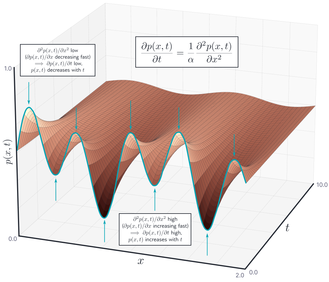
Figure 1.2 The heat equation. This is a partial differential equation where the dependent variable $p(x,t)$ is a probability distribution in $x$ for any given time $t$. The change in the probability distribution with $t$ depends on the second derivative with respect to $x$. Places where the gradient with respect to $x$ is increasing fast are pushed upwards as we move forwards in time and places where it is decreasing fast are pushed downwards.
The solution, which can be derived using the Fourier transform or other methods beyond the scope of this article is:
\begin{equation}
p(x,t) = \frac{1}{\sqrt{2\pi t}} \exp\left[-\frac{x^2}{2t}\right].
\tag{1.20}
\end{equation}
This is easy to confirm by computing the derivatives:
\begin{eqnarray}
\frac{\partial p(x,t)}{\partial t} &=& \frac{1}{\sqrt {2\pi}} \left(\frac{-t^{-3/2}}{2}\exp\left[-\frac{x^2}{2t}\right] + \frac{t^{-5/2}x^2}{2} \exp\left[-\frac{x^2}{2t}\right] \right)\nonumber \\
\frac{\partial^2 p(x,t)}{\partial x^2} &=& \frac{1}{\sqrt {2\pi}} \left(-t^{-3/2} \exp\left[-\frac{x^2}{2t}\right]+ t^{-5/2}x^2\exp\left[-\frac{x^2}{2t}\right] \right),
\tag{1.21}
\end{eqnarray}
which we can see by inspection conform to the PDE relation (equation 1.19). In terms of the PDE, the constant $1/\sqrt{2\pi}$ is arbitrary, but in practice this value is necessary to make this a valid probability distribution that integrates to one.
In our previous discussion of stochastic differential equations, we used the solution to $dx=dw$ as a base case and solved more complex SDEs by changing the variables until they fitted this form, using the known solution, and then transforming back again. In a very similar way, we can solve PDEs generated by the Fokker-Planck equation by changing the variables so that the PDE becomes a heat equation, solving that equation, and then transforming back again.
Solution of Ornstein-Uhlenbeck equation
Let’s exploit this approach to solve the Ornstein-Uhlenbeck equation:
\begin{equation}
dx = -\gamma x dt + \sigma dw.
\tag{1.22}
\end{equation}
The Fokker-Planck equation states that the distribution $p(x,t)$ evolves as:
\begin{equation}
\frac{\partial p(x,t)}{\partial t} = -\frac{\partial }{\partial x} \textrm{m}\bigl[x,t]p(x,t)+\frac{1}{2}\frac{\partial^2}{\partial x^2} s[x,t]^2 p(x,t).
\tag{1.23}
\end{equation}
where in this case $\mbox{m}[x,t] = -\gamma x$ and $s[x,t] = \sigma$. This gives us the partial differential equation:
\begin{equation}
\frac{\partial p(x,t)}{\partial t} = \gamma \frac{\partial }{\partial x} x p(x,t)+\frac{\sigma^2 }{2}\frac{\partial^2}{\partial x^2} p(x,t).
\tag{1.24}
\end{equation}
To solve this PDE, we will make two changes of variables which result in a heat equation. We solve that equation and transform back again to find the final expression for $p(x,t)$.
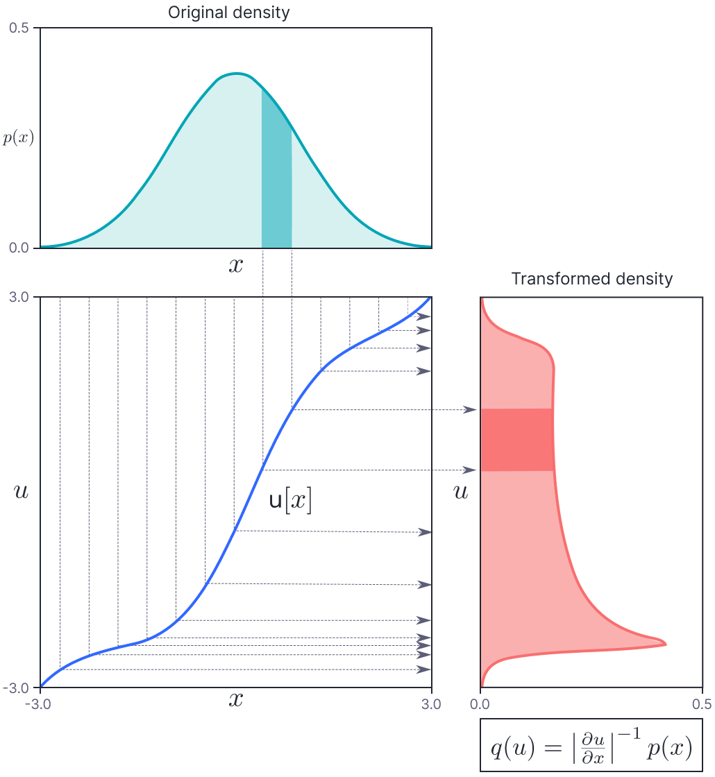
Figure 1.3 Change in variables. The original density $p(x)$ (cyan, top) passes through a function $\mbox{u}[x]$ (blue curve, bottom left) to create the transformed density $q(u)$ (orange, right). Consider dividing the base density into equal intervals (dashed vertical lines). The probability mass between adjacent lines must remain the same after transformation. The cyan-shaded region passes through a part of the function where the gradient is larger than one, so this region is stretched. Consequently, the height of the orange-shaded region must be lower so that it retains the same area as the cyan-shaded region. In other places (e.g., $x=2$), the gradient is less than one, and the model density increases relative to the base density. The rule for transforming the density is $q(u) = |\partial u/ \partial x|^{-1} p(x)$.
Step 1 — Change of variables: we first make the same change of variables $u = \exp[\gamma t] x$ that we did when we solved the SDE directly (see part VII of this series). It follows that $du=\exp[\gamma t]dx$ and $x=\exp[-\gamma t] u$. Using the change of variables formula for probability distributions (figure 1.3), we can find an expression for the probability distribution $q(u,t)$ over the new variable:
\begin{equation}
q(u,t) = \left|\frac{\partial u}{\partial x}\right|^{-1} p(x,t) =\exp[-\gamma t] p(x,t).
\tag{1.25}
\end{equation}
Now let’s use this change of variable in the Fokker-Planck partial differential equation. We have:
\begin{equation}
\frac{\partial p(x,t)}{\partial t} = \gamma \frac{\partial }{\partial x}\biggl( x \cdot p(x,t)\biggr)+\frac{\sigma^2 }{2}\frac{\partial^2}{\partial x^2} p(x,t).
\tag{1.26}
\end{equation}
Tackling the left-hand side of equation 1.26 first, we get:
\begin{eqnarray}
\frac{\partial p(x,t)}{\partial t} &=& \frac{\partial q(u,t)\exp[\gamma t]}{\partial t} \nonumber\\
&=& \left(\frac{\partial q(u,t)}{\partial t}+\frac{\partial q(u,t)}{\partial u}\frac{\partial u}{\partial t}\right)\exp[\gamma t]+\gamma q(u,t) \exp[\gamma t]\nonumber \\
&=& \left(\frac{\partial q(u,t)}{\partial t}+\frac{\partial q(u,t)}{\partial u}\gamma u \right)\exp[\gamma t]+\gamma q(u,t) \exp[\gamma t]\nonumber\\
&=& \left(\frac{\partial q(u,t)}{\partial t}+\frac{\partial q(u,t)}{\partial u}\gamma u +\gamma q(u,t) \right)\exp[\gamma t],
\tag{1.27}
\end{eqnarray}
where we have used the chain rule and the total derivative rule between lines one and two, the relations $\partial u/\partial t = \partial \exp[\gamma t]x/\partial t = \gamma \exp[\gamma t]x =\gamma u$ between lines two and three and tidied up the terms between lines three and four.
Now, we will work on the first term on the right-hand side of equation 1.26. We first consider the derivative:
\begin{eqnarray}
\frac{\partial p(x,t)}{\partial x} &=& \frac{\partial q(u,t)\exp[\gamma t]}{\partial x} \nonumber\\
&=& \frac{\partial q(u,t)\exp[\gamma t]}{\partial u}\frac{\partial u}{\partial x} \nonumber\\
&=& \frac{\partial q(u,t)\exp[\gamma t]}{\partial u} \exp[\gamma t]\nonumber \\
&=& \exp[2\gamma t]\frac{\partial q(u,t)}{\partial u},
\tag{1.28}
\end{eqnarray}
where we have used the chain rule between lines two and three, the relation $\partial u/\partial x = \partial \exp[\gamma t]x/\partial x = \exp[\gamma t]$ between lines two and three and tidied up between lines three and four. Then we find an expression for the first term on the right-hand side of equation 1.26 using the chain rule:
\begin{eqnarray}
\frac{\partial }{\partial x}x p(x,t) &=& p(x,t)+ x\cdot \frac{\partial p(x,t)}{\partial x}\nonumber \\
&=& \exp[\gamma t] q(u,t) + \exp[-\gamma t] u\cdot \exp[2\gamma t]\frac{\partial q(u,t)}{\partial u}\nonumber \\
&=& \left(q(u,t) + u \frac{\partial q(u,t)}{\partial u}\right)\exp[\gamma t].
\tag{1.29}
\end{eqnarray}
Finally, we compute the second term on the right-hand side of equation 1.26:
\begin{eqnarray}
\frac{\partial^2 p(x,t)}{\partial x^2} &=& \frac{\partial}{\partial x} \frac{\partial p(x,t)}{\partial x} \nonumber \\
&=& \frac{\partial}{\partial x} \exp[2\gamma t]\frac{\partial q(u,t)}{\partial u}\nonumber\\
&=& \frac{\partial}{\partial u} \exp[2\gamma t]\frac{\partial q(u,t)}{\partial u} \frac{\partial u}{\partial x} \nonumber \\
&=& \exp[3\gamma t]\frac{\partial^2 q(u,t)}{\partial u^2},
\tag{1.30}
\end{eqnarray}
where we have substituted in the expression derived in equation 1.28 between the first and second lines, used the chain rule between the second and third lines and tidied up between the third and fourth lines.
Now we substitute these three expressions into the original partial differential equation:
\begin{equation}
\frac{\partial p(x,t)}{\partial t} = \gamma \frac{\partial }{\partial x}\biggl( x \cdot p(x,t)\biggr)+\frac{\sigma^2 }{2}\frac{\partial^2}{\partial x^2} p(x,t),
\tag{1.31}
\end{equation}
to yield:
\begin{eqnarray}
\left(\frac{\partial q(u,t)}{\partial t}+\frac{\partial q(u,t)}{\partial u}\gamma u +\gamma q(u,t) \right)\exp[\gamma t] &=& \\
&&\hspace{-8cm}\gamma\left(q(u,t) + u \frac{\partial q(u,t)}{\partial u}\right)\exp[\gamma t]+\frac{\sigma^2}{2}\exp[3\gamma t]\frac{\partial^2 q(u,t)}{\partial u^2},\nonumber
\tag{1.32}
\end{eqnarray}
which after canceling out terms and dividing by $\exp[\gamma t]$ becomes:
\begin{equation}
\frac{\partial q(u,t)}{\partial t} = \frac{\sigma^2}{2}\exp[2\gamma t]\frac{\partial^2 q(u,t)}{\partial u^2}.
\tag{1.33}
\end{equation}
Step 2 — Second change of variables: This is almost the heat equation that we know the solution to (see the previous section). To massage it into this form, we make a second change of variable:
\begin{equation}
v = \frac{\sigma^{2}(\exp[2\gamma t] – 1)}{2\gamma} \implies \frac{\partial v}{\partial t} = \sigma^2\exp[2\gamma t].
\tag{1.34}
\end{equation}
We convert the left-hand side of equation 1.33 to use this new variable:
\begin{eqnarray}
\frac{\partial q(u,t)}{\partial t} &=& \frac{\partial q(u,v)}{\partial v}\frac{\partial v}{\partial t}\nonumber \\
&=& \frac{\partial q(u,v)}{\partial v} \sigma^2\exp[2\gamma t],
\tag{1.35}
\end{eqnarray}
where we have used the chain rule in the first line.
Substituting into 1.33, we have:
\begin{equation}
\frac{\partial q(u,v)}{\partial v}\sigma^2\exp[2\gamma t] = \frac{\sigma^2}{2}\exp[2\gamma t]\frac{\partial^2 q(u,v)}{\partial u^2},
\tag{1.36}
\end{equation}
which gives the equation:
\begin{equation}
\frac{\partial q(u,v)}{\partial v} = \frac{1}{2}\frac{\partial^2 q(u,v)}{\partial u^2},
\tag{1.37}
\end{equation}
Step 3 — Solve the heat equation: As in the previous section, the solution to this heat equation for initial conditions $q(u,0) = \delta[u-x_0]$ which implies:
\begin{equation}
q(u,v) = \frac{1}{\sqrt{2\pi v}}\exp\left[-\frac{(u-x_0)^2}{2v}\right].
\tag{1.38}
\end{equation}
Step 4 — Substitute back in the original variables: First we substitute back in $v = \sigma^2(\exp[2\gamma t] – 1)/2\gamma$:
\begin{equation}
q(u,t) = \frac{1}{\sqrt{2\pi \sigma^2\bigl(\exp[2\gamma t] -1\bigr)/2\gamma}}\exp\left[-\frac{\bigl( u-x_0\bigr)^2}{2\sigma^2 (\exp[2\gamma t]-1)/2\gamma}\right].
\tag{1.39}
\end{equation}
Then we return to $p(x,t)$ using $u=\exp[\gamma t] x$ and the change of variables relation $p(x,t)=\exp[\gamma t] q(u,t)$ from equation 1.25:
\begin{eqnarray}
p(x,t) &=& \frac{\exp[\gamma t]}{\sqrt{2\pi \sigma^2\bigl(\exp[2\gamma t] -1\bigr)/2\gamma}}\exp\left[-\frac{ \bigl( \exp[\gamma t] x-x_0\bigr)^2}{2\sigma^2 (\exp[2\gamma t]-1)/2\gamma}\right]\\
&=& \frac{\exp[\gamma t]}{\sqrt{2\pi \sigma^2\bigl(\exp[2\gamma t] -1\bigr)/2\gamma}}\exp\left[-\frac{ \exp[2\gamma t]\bigl( x-x_0\exp[-\gamma t]\bigr)^2}{2\sigma^2 (\exp[2\gamma t]-1)/2\gamma}\right]\nonumber\\
&=&\frac{1}{\sqrt{2\pi \sigma^2\bigl(1-\exp[-2\gamma t]\bigr)/2\gamma}}\exp\left[-\frac{ \bigl( x-x_0\exp[-\gamma t]\bigr)^2}{2\sigma^2 (1-\exp[-2\gamma t])/2\gamma}\right]\nonumber.
\tag{1.40}
\end{eqnarray}
We can now see by inspection that:
\begin{equation}
p(x,t) \sim \mbox{Norm}_{x}\left[x_0\exp[-\gamma t], \frac{\sigma^2}{2\gamma}\Bigl(1-\exp[-2\gamma t]\Bigr)\right].
\tag{1.41}
\end{equation}
which is exactly the same result we got in part VII of this series when we solved the SDE using Itô’s lemma.
Conclusion
The Fokker-Planck equation converts an SDE in a variable $x[t]$ into a partial differential equation in the probability distribution $p(x,t)$ over that variable. Solving this PDE is an alternative approach to solving the SDE directly. To demonstrate this, we derived the Fokker-Planck PDE for the Ornstein-Uhlenbeck process, solved this PDE, and saw that we got the same result as when we solved this SDE directly. The Fokker-Planck equation is also a useful tool in its own right; in the following section, we use this to prove Anderson’s reverse-time theorem.
Reverse-time ODEs and SDEs
Consider an ODE with the form:
\begin{equation}
p(x,t) \sim \mbox{Norm}_{x}\left[x_0\exp[-\gamma t], \frac{\sigma^2}{2\gamma}\Bigl(1-\exp[-2\gamma t]\Bigr)\right].
\tag{1.42}
\end{equation}
We have seen that we can extrapolate from a given initial condition $x_0$ by either finding a closed-form solution for the ODE, or propagating it forward numerically. This section considers what happens if we want to propagate the ODE backwards in time. In other words, we are given some boundary condition $x_T$, and want to know how the function wound up arriving at this point.
Since ODEs are deterministic, this turns out to be very simple; there is a one-to-one map between the value at one time and the value at any time in the future. The reverse-time equation just multiplies the function $\mbox{m}[x,t]$ by minus one (figure 1.4a-b):
\begin{equation}
d\overline{x} = -\mbox{m}[\overline{x},t] dt,
\tag{1.43}
\end{equation}
where the notation $d\overline{x}$ denotes that we are moving backwards in time.
Now consider an SDE of the form:
\begin{equation}
dx = \mbox{m}[x,t] dt + \mbox{s}[x,t]dw,
\tag{1.44}
\end{equation}
with some initial condition $x_0$. Consider what would happen if we propagated the solution forward to time $T$, and then naïvely propagated backwards using the same approach of multiplying the terms by minus one:
\begin{eqnarray}
d\overline{x} &=& -\textrm{m}\bigl[\overline{x},t\bigr] dt – \textrm{s}\bigl[\overline{x},t\bigr] dw,
\tag{1.45}
\end{eqnarray}
where we have multiplied both terms by minus one. Do you think that the solutions will correctly converge back to the initial condition $x_0$?
In fact, the mean of the solution propagates backwards correctly, but example paths do not converge back to the initial value (figure 1-4c-d); they diverge further. Careful consideration of the diffusion term $\textrm{s}\bigl[x,t\bigr] dw$ reveals that this is unsurprising. The definition of $dw$ is $\lim_{\Delta t \rightarrow 0} \sqrt{\Delta t} z_t$ where $z_t$ is a draw from a standard normal distribution. This distribution is symmetric about zero, so multiplying the draw by minus one has no effect. Whether the sign of the $dw$ term is positive or negative, the result is that noise is added and individual paths diverge.
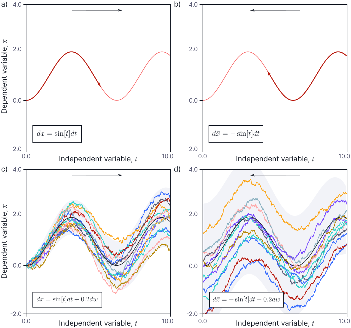
Figure 1.4 Reverse-time ODEs and SDEs. a) The forward ODE propagates a value $x$ forward in time. b) The matching reverse ODE (which is just the original ODE multiplied by a factor of minus one) propagates the value back in time along the same trajectory. c) A forward SDE propagates a value $x$ forward in time but includes a diffusion (noise) term that means the result is different every time. The solution of the SDE is denoted by the gray region representing $\pm 2$ standard deviations of the marginal distributions. d) If we naïvely multiply the terms in the SDE by minus one, the SDE does not reverse correctly; the paths do not converge back to the initial condition $x_0 = 0$, and the marginal distributions (gray region) do not match the forward process.
Anderson’s theorem
Anderson’s theorem defines a reverse-time SDE that has the same marginal distributions as the forward process (but not necessarily the same joint distribution). If the forward time process is given by:
\begin{equation}
dx = \mbox{m}[x, t] dt + \mbox{s}[x,t] dw,
\tag{1.46}
\end{equation}
with initial condition $x_{0}\sim p_0(x)$, then the reverse-time SDE is given by:
\begin{equation}
d\overline{x} = -\left(\textrm{m}\bigl[\overline{x},t]-\textrm{s}[\overline{x},t]^2\frac{d\log \bigl[p(\overline{x}|t)\bigr]}{d\overline{x}}\right)dt + \mbox{s}[\overline{x},t]dw,
\tag{1.47}
\end{equation}
with initial condition $x_{T}\sim p_T(\overline{x})$. In this expression, the term $p(\overline{x}|t)$ denotes the marginal distribution of the solution of the forward SDE at time $t$.
This is illustrated in figure 1.5. Anderson’s modified reverse equation has the same diffusion term as the forward equation, but a drift term that gradually forces the paths to re-converge to the initial condition. The more that a path deviates from what is typical (i.e., the lower the probability), the stronger the tendency of the drift term to force the path back towards the mean.
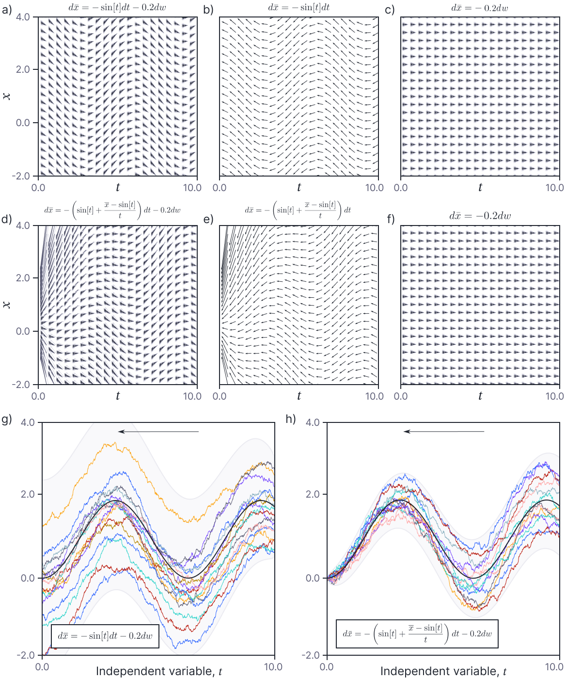
Figure 1.5 Anderson’s reverse-time theorem. a) Naïve reverse SDE visualized as a flow field, b) drift term only and c) diffusion term only. This SDE has solution $p(x,t)\sim \mbox{Norm}_{x}[\sin[t], t]$. d) Anderson’s modified reverse-time SDE visualized as a flow field. e) Drift term only. f) Diffusion term only. g) Solution and example paths of naïve reverse SDE. The paths diverge and the marginal distributions of the solution (gray region) does not match the forward SDE. h) Solution and example paths of modified SDE; the paths all converge back to the starting point and the marginal distributions of the solution match the forward SDE.
Confirmation of Anderson’s theorem
We’ll exploit the Fokker-Planck equation to show that Anderson’s theorem is true for the case where the diffusion term depends on $t$ alone. Our approach will be to convert both the forward SDE and Anderson’s reverse-time SDE to a PDE in the probability distribution and show that this PDE is the same in both cases.
To this end, we first consider the forward SDE:
\begin{equation}
dx = \textrm{m}\bigl[x,t] dt + s[t] dw,
\tag{1.48}
\end{equation}
where $x_{0} \sim p_0(x)$. The associated marginal densities $p(x|t)$ must satisfy the Fokker-Planck equation:
\begin{equation}
\frac{\partial p(x|t)}{\partial t} = -\frac{\partial }{\partial x} \textrm{m}\bigl[x,t]p(x|t)+\frac{1}{2}\frac{\partial^2}{\partial x^2} s[t]^2 p(x|t).
\tag{1.49}
\end{equation}
Now consider Anderson’s reverse-time SDE:
\begin{equation}
d\overline{x} = -\left(\textrm{m}\bigl[\overline{x},t]-\textrm{s}[t]^2\frac{d\log \bigl[p(\overline{x}|t)\bigr]}{d\overline{x}}\right)dt + \mbox{s}[t]dw.
\tag{1.50}
\end{equation}
which would have marginal densities $p(\overline{x}|t)$ that satisfy the reverse Fokker-Planck equation:
\begin{equation}
\frac{\partial p(\overline{x}|t)}{\partial t} = \frac{\partial }{\partial \overline{x}} \left(\textrm{m}\bigl[\overline{x},t]-\textrm{s}[t]^2\frac{d\log \bigl[p(\overline{x}|t)\bigr]}{d\overline{x}}\right)p(\overline{x}|t)-\frac{1}{2}\frac{\partial^2}{\partial \overline{x}^2} \textrm{s}[t]^2 p(\overline{x}|t).
\tag{1.51}
\end{equation}
To prove that Anderson’s theorem is correct, we need to show that the marginal distributions $p(x|t)$ in equation 1.49 are updated in the opposite way to the marginal distributions $p(\overline{x}|t)$ in equation 1.51.
To this end, we manipulate equation 1.51:
\begin{align}
\hspace{-1cm}\frac{\partial p(\overline{x}|t)}{\partial t}\hspace{1cm} &\hspace{-1cm}= -\frac{\partial }{\partial \overline{x}} \left(\textrm{m}\bigl[\overline{x},t]-\textrm{s}[t]^2\frac{d\log \bigl[p(\overline{x}|t)\bigr]}{d\overline{x}}\right)p(\overline{x}|t)-\frac{1}{2}\frac{\partial^2}{\partial \overline{x}^2} \textrm{s}\bigl[t\bigr]^2 p(\overline{x}|t)\nonumber \\
&\hspace{-1cm}= -\frac{\partial }{\partial \overline{x}} \left(\textrm{m}\bigl[\overline{x},t]-\textrm{s}[t]^2\frac{d p(\overline{x}|t)\bigr]}{d\overline{x}}\cdot \frac{1}{p(\overline{x}|t)}\right)p(\overline{x}|t)-\frac{1}{2}\frac{\partial^2}{\partial \overline{x}^2} \textrm{s}\bigl[t]^2 p(\overline{x}|t)\nonumber \\
&\hspace{-1cm}= -\frac{\partial}{\partial \overline{x}} \left(\textrm{m}\bigl[\overline{x},t]p(\overline{x}|t) -\textrm{s}[t]^2\frac{d p(\overline{x}|t)\bigr]}{d\overline{x}|t}\right)-\frac{1}{2}\frac{\partial^2}{\partial \overline{x}^2} \textrm{s}\bigl[t]^2 p(\overline{x})\nonumber \\
&\hspace{-1cm}= -\frac{\partial}{\partial \overline{x}} \textrm{m}\bigl[\overline{x},t]p(\overline{x}|t) +\frac{1}{2}\frac{\partial^2}{\partial \overline{x}^2} \textrm{s}\bigl[t\bigr]^2 p(\overline{x}|t),
\tag{1.52}
\end{align}
where we have used the chain rule between lines one and two, canceled terms $p(\overline{x}|t)$ between lines two and three and combined the last two terms between lines three and four. The result is the same as the PDE for the forward evolution of the probability distribution (equation 1.49) as required. Note that Anderson’s theorem is true for the more complex case where the diffusion term $s[x,t]$ depends on both $x$ and $t$, but the proof requires a different style of argument that is beyond the scope of this book.
Discussion
This article described the Fokker-Planck equation which allows us to map an SDE in some variable $x$ to an equivalent PDE over the probability distribution $p(x,t)$ of that variable. This admitted a different method for solving SDEs. We also discussed Anderson’s reverse-time theorem, which allows us to reverse the direction of SDEs such that the marginal distributions of the reverse equation match those of the forward equation. We used the Fokker-Planck equation to prove that these marginal distributions are identical.
This concludes our discussion of SDEs and ODEs in the abstract. Subsequent articles in this series apply these ideas to machine learning. We start by considering the limit of gradient descent as the learning rate becomes zero as an ODE and the limit of stochastic gradient descent as an SDE.