
This is Part IX of a series of articles about the use of ordinary differential equations (ODEs) and stochastic differential equations (SDEs) in machine learning. Part I of this series provided an overview of this area. Part II, Part III, and Part IV presented background material on ODEs and Part V, Part VI, Part VII, and Part VIII presented background material on SDEs. The remaining articles in this series apply these ideas to different aspects of machine learning.
In this article we consider the use of gradient descent and stochastic gradient descent for learning model parameters. With an infinitesimal step size gradient descent becomes an ODE and stochastic gradient descent becomes an SDE. We analyze the SDE associated with stochastic gradient descent to help understand how batch size and step size trade-off during optimization. The SDE formulation also throws light on how the final expected loss relates to the width of the minimum at convergence.
Then we return to the practical case of finite step sizes. We characterize the deviation from the infinitesimal case as an additive regularization term. This is known as implicit regularization. This explains why larger learning rates and smaller batches lead to better generalization (figure 1.1).
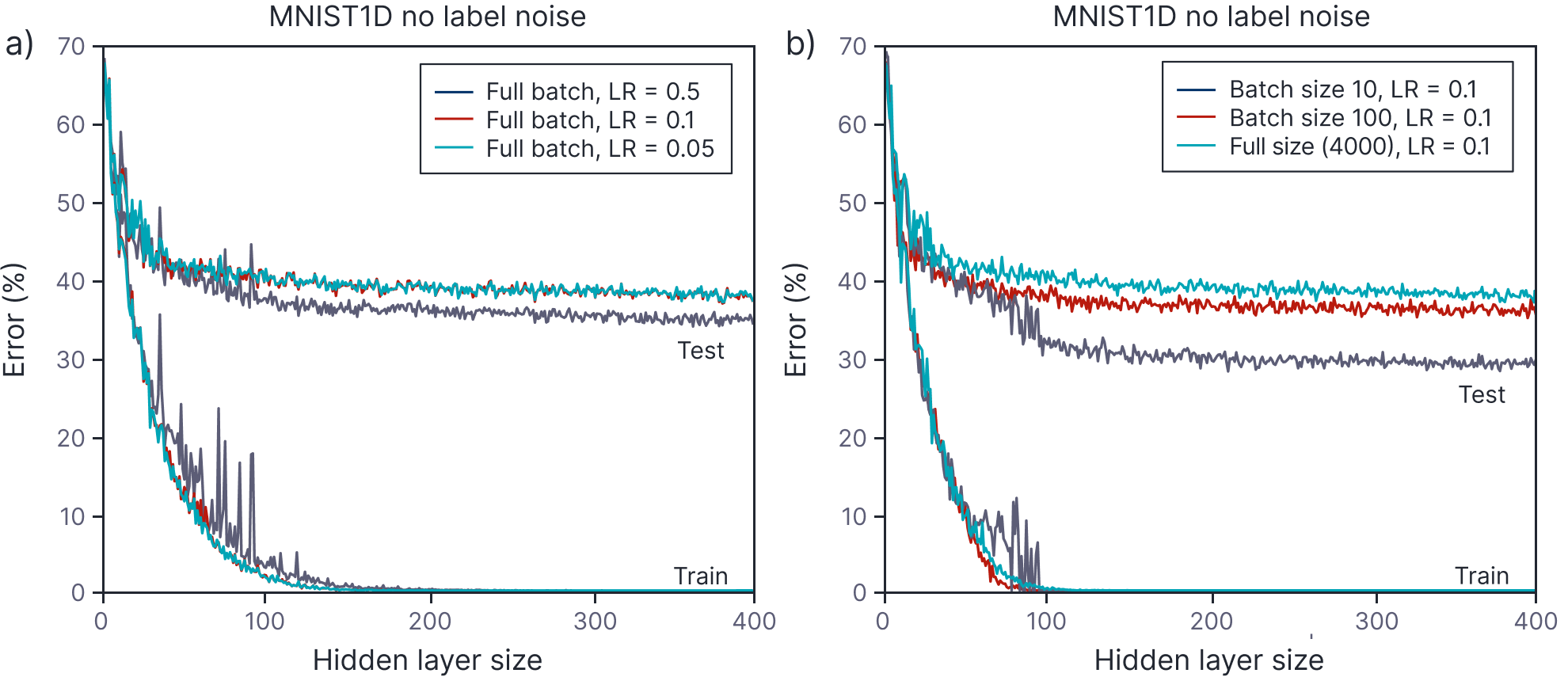
Figure 1.1 Effect of learning rate (LR) and batch size for 4000 training and 4000 test examples from MNIST-1D for a neural network with two hidden layers. a) Performance is better for large learning rates than for intermediate or small ones. In each case, the number of iterations is 6000$/$LR, so each solution has the opportunity to move the same distance. b) Performance is superior for smaller batch sizes. In each case, the number of iterations was chosen so that the training data were memorized at roughly the same model capacity. Adapted from Prince (2023).
Gradient descent as an ODE
Consider a machine learning model with parameters $\boldsymbol\phi$ that is trained using $I$ input/output pairs $\{\mathbf{x}_{i},\mathbf{y}_i\}$. We write the loss for the $i^{th}$ data point as $\ell[\mathbf{x}_i, \mathbf{y}_i, \boldsymbol\phi]$, or $\ell_i$ for short, and the total loss as $L= \frac{1}{I}\sum_i \ell_i$. Consider training this model with gradient descent with step size $\alpha$. The parameters at time step $k$ evolve according to the relation:
\begin{equation}
\boldsymbol\phi_{k+1} = \boldsymbol\phi_{k} – \alpha \cdot \textbf{g}[\boldsymbol\phi_k],
\tag{1.1}
\end{equation}
where the gradient $\textbf{g}[\boldsymbol\phi]$ is the average of the gradients of the individual loss terms:
\begin{equation}
\textbf{g}[\boldsymbol\phi]= \frac{1}{I}\sum_{i=1}^I\frac{\partial \ell_i}{\partial \boldsymbol\phi}.
\tag{1.2}
\end{equation}
The gradient update can be re-arranged to:
\begin{equation}
\boldsymbol\phi_{k+1} – \boldsymbol\phi_{k} = -\alpha \cdot \textbf{g}[\boldsymbol\phi_k].
\tag{1.3}
\end{equation}
Now we define $\Delta t=\alpha$ and move to continuous time $t=k\Delta t$:
\begin{equation}
\boldsymbol\phi_{t+\Delta t} – \boldsymbol\phi_{t} = -\Delta t \cdot \textbf{g}[\boldsymbol\phi_t],
\tag{1.4}
\end{equation}
We take the limit:
\begin{equation}
\frac{\boldsymbol\phi_{t+\Delta t} – \boldsymbol\phi_{t} }{\Delta t} \longrightarrow \frac{d \boldsymbol \phi}{d t} \quad\quad\quad \mbox{as }\quad\quad\quad\Delta t \longrightarrow 0,
\tag{1.5}
\end{equation}
which gives us:
\begin{equation}
\frac{d\boldsymbol\phi}{dt} = – \textbf{g}[\boldsymbol\phi_t].
\tag{1.6}
\end{equation}
This ODE is known as the gradient flow equation. It determines how the parameters would evolve in the ideal case where we used an infinitesimal step size (figure 1.2).
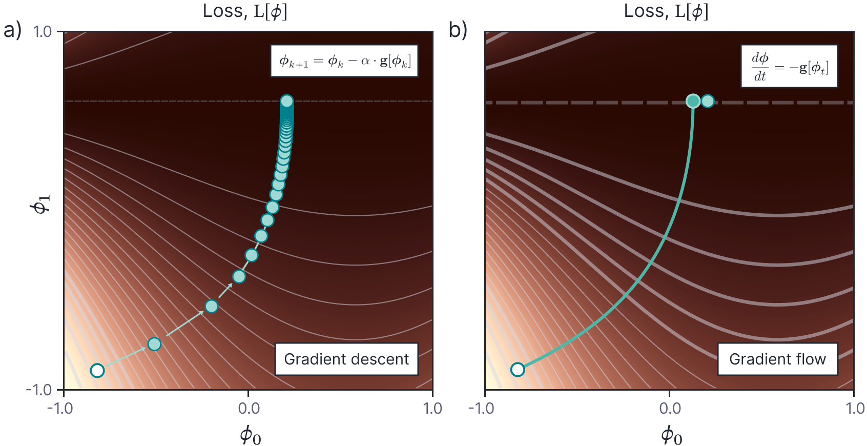
Figure 1.2 Gradient descent vs. gradient flow. a) Gradient descent proceeds by measuring the gradient at a point and then moving a fixed distance in that direction, where the distance is the product of the magnitude of the gradient and a learning rate $\alpha$. b) Gradient flow is the limit of this process as the learning rate becomes infinitesimal; here the trajectory of the parameters is governed by an ODE and becomes smooth. Note that the final position reached by gradient descent may not be the same as for gradient flow. The finite learning rate means that gradient descent does not proceed neutrally to a minimum but exhibits a bias relative to gradient flow. We return to this point later in this article when we cast this in terms of implicit regularization.
Stochastic gradient descent as an SDE
Stochastic gradient descent can similarly be written as:
\begin{equation}
\boldsymbol\phi_{k+1} – \boldsymbol\phi_{k} = – \alpha \cdot \textbf{g}^{s}[\boldsymbol\phi_k],
\tag{1.7}
\end{equation}
where the batch gradient $\textbf{g}^{s}[\boldsymbol\phi_k]$ at step $k$ is:
\begin{equation}
\textbf{g}^{s}[\boldsymbol\phi_k] = \frac{1}{|\mathcal{B}|}\sum_{i\in \mathcal{B}_{k}}\frac{\partial \ell_i}{\partial \boldsymbol\phi}.
\tag{1.8}
\end{equation}
Here, $\boldsymbol\phi$ are the model parameters, $\alpha$ is the learning rate, $\mathcal{B}_k$ is the set of indices in the $k^{th}$ batch, which is of size $|\mathcal{B}|$, and $\ell_i$ is the $i^{th}$ loss term.
Combining these equations yields:
\begin{equation}
\boldsymbol\phi_{k+1} – \boldsymbol\phi_{k} = – \frac{\alpha}{|\mathcal{B}|} \cdot \sum_{i\in \mathcal{B}_{k}}\frac{\partial \ell_i}{\partial \boldsymbol\phi}.
\tag{1.9}
\end{equation}
We can rewrite this as the full gradient update plus the difference from that update:
\begin{eqnarray}\label{eq:ode9_will_be_sde}
\boldsymbol\phi_{k+1} – \boldsymbol\phi_{k} &=& -\alpha \cdot \frac{1}{I} \sum_{i=1}^I \frac{\partial \ell_i}{\partial \boldsymbol\phi}-\alpha\left(\frac{1}{|\mathcal{B}|}\sum_{i\in \mathcal{B}} \frac{\partial \ell_i}{\partial \boldsymbol\phi}-\frac{1}{I}\sum_{i=1}^I \frac{\partial \ell_i}{\partial \boldsymbol\phi}\right)\nonumber \\
&=& -\alpha \cdot \textbf{g}[\boldsymbol\phi] – \alpha \cdot \boldsymbol\epsilon,
\tag{1.10}
\end{eqnarray}
where we have added and subtracted the full gradient in the first line and denoted the difference between the SGD update and that of full gradient descent by $\boldsymbol\epsilon$. The first term $\textbf{g}[\boldsymbol\phi]$ in equation 1.10 is deterministic, but the difference term $\boldsymbol\epsilon$ is stochastic; it depends on the random assignment of the data points to this batch.
The mean of the difference term is zero; the batch gradient is on average the same as the gradient from the full dataset. Our goal now is to characterize the covariance of this difference term, which will allow us to derive the noise term of the associated SDE.
Mean and covariance of individual gradients
We start by considering the moments of the individual gradient $\partial \ell_i/ \partial \boldsymbol\phi$. We’ll use these when we find an expression for the covariance of $\epsilon$. The mean of $\partial \ell_i/ \partial \boldsymbol\phi$ is the full gradient:
\begin{equation}
\mathbb{E}\left[\frac{\partial \ell_i}{\partial \boldsymbol\phi} \right]=\textbf{g}[\boldsymbol\phi].
\tag{1.11}
\end{equation}
This is not surprising; the gradient was originally defined as the average of the individual gradients $\textbf{g}[\boldsymbol\phi]=(1/I)\sum_i \partial \ell_i/\partial \boldsymbol\phi$. For any set of parameters $\boldsymbol\phi$, the covariance of the individual gradient has some value $\boldsymbol\Sigma[\boldsymbol\phi]$ so we can write:
\begin{equation}\label{eq:ode9_individual_moment1}
\mbox{Cov}\left[\frac{\partial \ell_i}{\partial \boldsymbol\phi} \right]=\boldsymbol\Sigma[\boldsymbol\phi].
\tag{1.12}
\end{equation}
This is illustrated in figure 1.3.
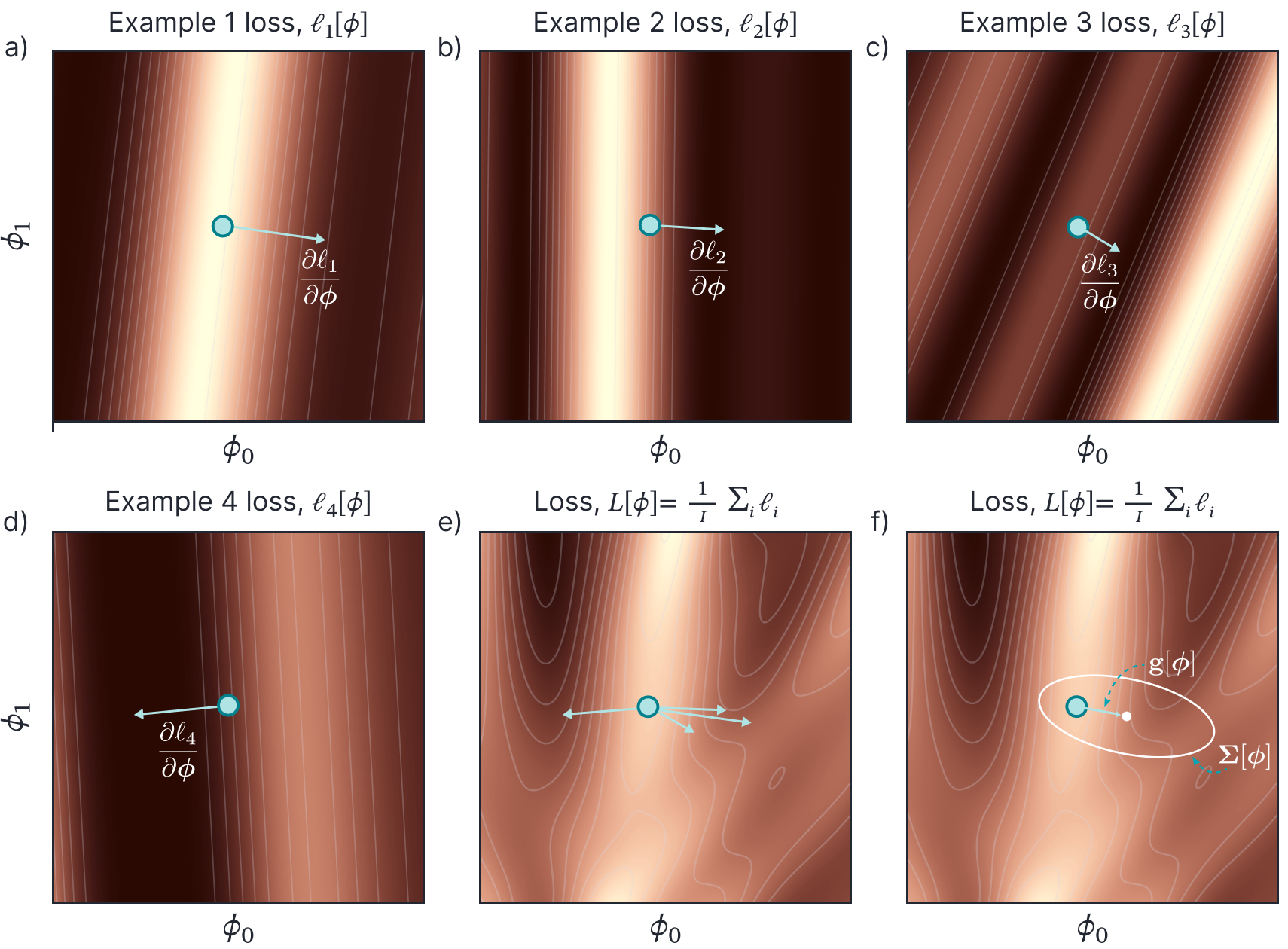
Figure 1.3 Mean and covariance of individual loss terms. a) Heatmap shows the loss function for the first data point. Consider some fixed value of the parameters $\boldsymbol\phi$ (cyan circle). The gradient $\partial \ell_1/\partial \boldsymbol\phi$ is illustrated by the arrow. b-d) Each different data example corresponds to a different individual loss function and a different gradient. e) Together these gradients have some distribution, which f) can be characterized by a normal distribution with mean $\textbf{g}[\boldsymbol\phi]$ and covariance $\boldsymbol\Sigma[\boldsymbol\phi]$.
It follows that the second moment around zero can be written as:
\begin{equation}\label{eq:ode9_individual_moment2}
\mathbb{E}\left[\frac{\partial \ell_i}{\partial \boldsymbol\phi}\frac{\partial \ell_j}{\partial \boldsymbol\phi}^T\right] = \begin{cases}
\textbf{g}[\boldsymbol\phi]\textbf{g}[\boldsymbol\phi]^T & i\neq j \\
\textbf{g}[\boldsymbol\phi]\textbf{g}[\boldsymbol\phi]^T +\boldsymbol\Sigma[\boldsymbol\phi] & i = j
\end{cases}.
\tag{1.13}
\end{equation}
Here we have exploited the variance identity: $
\mathbb{E}[(\mathbf{z}-\boldsymbol\mu_z)(\mathbf{z}-\boldsymbol\mu_z)^T] = \mathbb{E}[\mathbf{z}\mathbf{z}^T] – \boldsymbol\mu_z\boldsymbol\mu_z^T$. There are two cases because we are assuming that the samples are drawn independently; the covariance of samples with different indices is zero, but the covariance of samples with the same index is non-zero and is characterized by $\boldsymbol\Sigma[\boldsymbol\phi]$.
Mean and covariance of batch
We now use the results from equations 1.12 and 1.13 to derive expressions for the mean $\boldsymbol\mu_{\boldsymbol\epsilon}$ and covariance $\boldsymbol\Sigma_{\boldsymbol\epsilon}$ of the difference term $\boldsymbol\epsilon$. For the mean we have:
\begin{eqnarray}
\boldsymbol\mu_{\boldsymbol\epsilon} &=& \mathbb{E}\left[\frac{1}{|\mathcal{B}|}\sum_{i\in \mathcal{B}} \frac{\partial \ell_i}{\partial \boldsymbol\phi}-\frac{1}{I}\sum_{i=1}^I \frac{\partial \ell_i}{\partial \boldsymbol\phi}\right]\nonumber\\
&=& \frac{1}{|\mathcal{B}|}\mathbb{E}\left[\sum_{i\in \mathcal{B}} \frac{\partial \ell_i}{\partial \boldsymbol\phi}\right]-\frac{1}{I}\mathbb{E}\left[\sum_{i=1}^I \frac{\partial \ell_i}{\partial \boldsymbol\phi}\right]\nonumber\\
&=& \textbf{g}[\boldsymbol\phi]-\textbf{g}[\boldsymbol\phi] = \mathbf{0}.
\tag{1.14}
\end{eqnarray}
This is reassuring; we expect the stochastic gradient term to equal the full gradient term on average.
For the covariance, we have:
\begin{align}\label{eq:ode9_batch_covariance}
\hspace{-2cm}\boldsymbol\Sigma_{\boldsymbol\epsilon} \hspace{1cm}&\hspace{-1cm}= \mathbb{E}\left[\left(\frac{1}{|\mathcal{B}|}\sum_{i\in \mathcal{B}} \frac{\partial \ell_i}{\partial \boldsymbol\phi}-\frac{1}{I}\sum_{i=1}^I \frac{\partial \ell_i}{\partial \boldsymbol\phi}\right)\left(\frac{1}{|\mathcal{B}|}\sum_{i\in \mathcal{B}} \frac{\partial \ell_i}{\partial \boldsymbol\phi}-\frac{1}{I}\sum_{i=1}^I \frac{\partial \ell_i}{\partial \boldsymbol\phi}\right)^T\right]\nonumber \\
&= \frac{1}{|\mathcal{B}|^2}\sum_{i\in \mathcal{B}}\sum_{j\in \mathcal{B}}\mathbb{E}\left[ \frac{\partial \ell_i}{\partial \boldsymbol\phi} \frac{\partial \ell_j}{\partial \boldsymbol\phi}^T\right] -\frac{2}{I|\mathcal{B}|} \sum_{i\in \mathcal{B}}\sum_{j=1}^I\mathbb{E}\left[ \frac{\partial \ell_i}{\partial \boldsymbol\phi} \frac{\partial \ell_j}{\partial \boldsymbol\phi}^T\right]\nonumber\\
&\hspace{7cm}+\frac{1}{I^2}\sum_{i=1}^I\sum_{j=1}^I \mathbb{E}\left[ \frac{\partial \ell_i}{\partial \boldsymbol\phi} \frac{\partial \ell_j}{\partial \boldsymbol\phi}^T\right]\nonumber \\
&= \mathbf{g}[\boldsymbol\phi]\mathbf{g}[\boldsymbol\phi]^T – 2 \mathbf{g}[\boldsymbol\phi]\mathbf{g}[\boldsymbol\phi]^T\! +\! \mathbf{g}[\boldsymbol\phi]\mathbf{g}[\boldsymbol\phi]^T \!+\! \frac{1}{|\mathcal{B}|}\boldsymbol\Sigma[\boldsymbol\phi] – \frac{2}{I}\boldsymbol\Sigma[\boldsymbol\phi] \!+\! \frac{1}{I}\boldsymbol\Sigma[\boldsymbol\phi]\nonumber \\
&= \left(\frac{1}{|\mathcal{B}|} -\frac{1}{I}\right)\boldsymbol\Sigma[\boldsymbol\phi],
\tag{1.15}
\end{align}
where the last three terms in line three come from extracting the $|\mathcal{B}|$, $|\mathcal{B}|$, and $I$ terms where $i\!=\!j$ from the three terms in line two. This result is illustrated in figure 1.4.
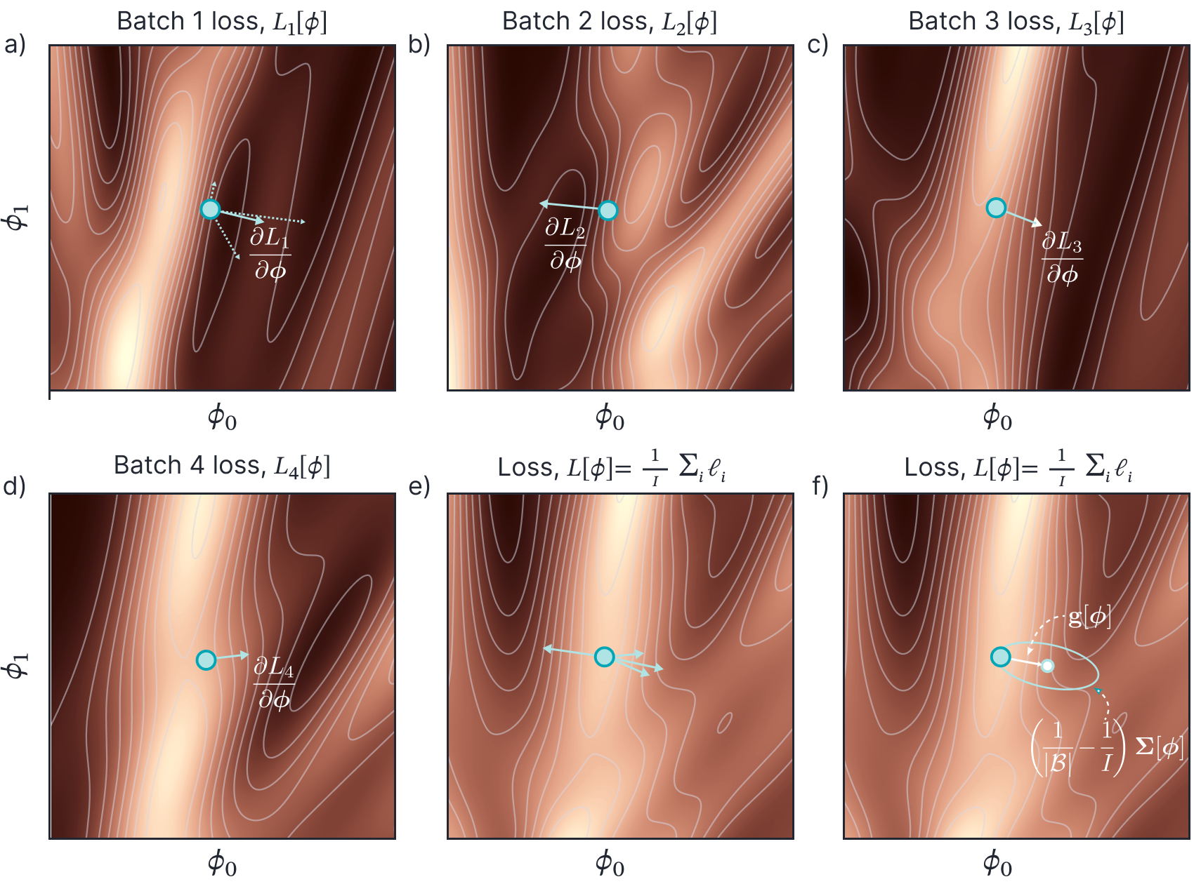
Figure 1.4 Mean and covariance of batch loss. a) Heatmap represents loss function $L_1[\boldsymbol\phi]$ for the first batch of size three. This is the average of the three individual loss functions of the constituent points (see figure 1.3). The gradient $\partial L_1/\partial \boldsymbol\phi$ (solid arrow) for some fixed parameters $\boldsymbol\phi$ (cyan circle) is the average of the gradients of the individual loss terms (dashed arrows). b-d) The gradients for batches two, three, and four are computed in the same way. e) Together these gradients have some distribution, which f) can be characterized by a normal distribution with mean $\textbf{g}[\boldsymbol\phi]$ and covariance $\boldsymbol\Sigma_\epsilon$.
Stochastic gradient flow
We’ll now use this result to derive the SDE that corresponds to stochastic gradient descent in the infinitesimal limit. We first make the assumption that the difference term $\boldsymbol\epsilon$ is distributed as a multivariate normal distribution and reinterpret equation 1.10 in terms of adding Gaussian noise:
\begin{eqnarray}
\boldsymbol\phi_{k+1} – \boldsymbol\phi_{k} &=&
-\alpha \cdot \textbf{g}[\boldsymbol\phi] – \alpha \cdot \boldsymbol\epsilon\nonumber \\
&=&-\alpha \cdot \textbf{g}[\boldsymbol\phi] – \alpha \cdot \sqrt{\frac{1}{|\mathcal{B}|} -\frac{1}{I}} \cdot \boldsymbol\Sigma[\boldsymbol\phi_k]^{1/2} \mathbf{z}_k,\nonumber
\end{eqnarray}
where $\mathbf{z}_k$ is a draw from a standard multivariate normal distribution. In the second line, we have used the standard method for drawing a sample from a multivariate normal distribution.
As in our treatment of gradient descent, we now move to continuous time $t=k\alpha = k\Delta t$, which yields:
\begin{equation}
\boldsymbol\phi_{t+\Delta t} – \boldsymbol\phi_{t} = – \Delta t \cdot \textbf{g}[\boldsymbol\phi_t] + \Delta t \cdot \sqrt{\frac{1}{|\mathcal{B}|} -\frac{1}{I}} \cdot \boldsymbol\Sigma[\boldsymbol\phi_t]^{1/2}\mathbf{z}_t,
\tag{1.16}
\end{equation}
Now we write $\Delta \boldsymbol\phi = \boldsymbol\phi_{t+\Delta t} – \boldsymbol\phi_{t}$ and write $\Delta t =\sqrt{\Delta t}\cdot \sqrt{\Delta t} = \sqrt{\alpha}\cdot \sqrt{\Delta t}$ to yield:
\begin{equation}
\Delta \boldsymbol\phi = – \textbf{g}[\boldsymbol\phi_t] \Delta t + \sqrt{\frac{\alpha}{|\mathcal{B}|} -\frac{\alpha}{I}} \cdot \boldsymbol\Sigma[\boldsymbol\phi_t]^{1/2} \left(\sqrt{\Delta t}\mathbf{z}_t\right).
\tag{1.17}
\end{equation}
As the time interval becomes infinitesimal, we have $\Delta \boldsymbol\phi \rightarrow d\boldsymbol\phi$, $\Delta t\rightarrow dt$, and $\sqrt{\Delta t}\mathbf{z}_t\rightarrow d\mathbf{w}_t$, which yields the stochastic differential equation:
\begin{equation}\label{eq:ode9_sde1}
d\boldsymbol\phi = – \textbf{g}[\boldsymbol\phi]dt +
\sqrt{\frac{\alpha}{|\mathcal{B}|} -\frac{\alpha}{I}} \cdot \boldsymbol\Sigma^{1/2}d\mathbf{w},
\tag{1.18}
\end{equation}
where $d\mathbf{w}_t$ is the is in infinitesimal increment of the Wiener process. This is termed the stochastic gradient flow equation (figure 1.5) and is equivalent to the gradient flow equation for standard gradient descent; it governs how stochastic gradient descent evolves in the ideal case of infinitesimal step size. Note that this derivation is based on that of Smith and Le (2018).
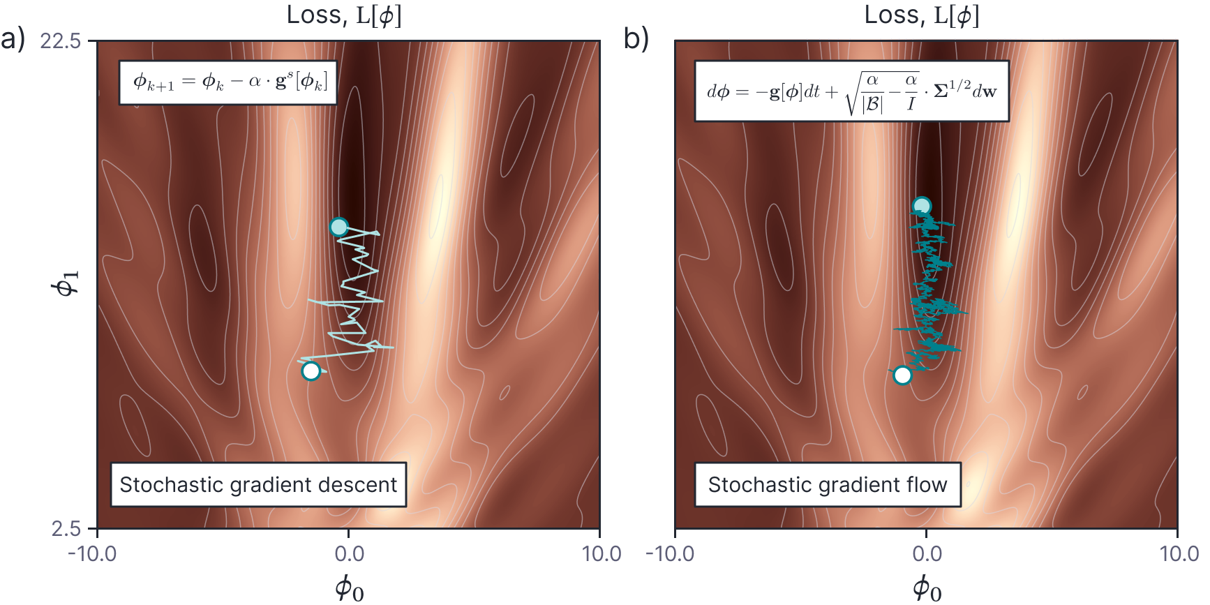
Figure 1.5 Stochastic gradient descent vs. stochastic gradient flow. a) Stochastic gradient descent proceeds by measuring the gradient at a point for the current batch and then moving a fixed distance in that direction, where the distance is the product of the magnitude of the gradient and a learning rate $\alpha$. Since the batch only consists of some of the data points, the direction does not necessarily align with the gradient of the global loss function $L[\boldsymbol\phi]$. b) Stochastic gradient flow is the limit of this process as the learning rate becomes infinitesimal. This SDE creates a path through the parameter space that is stochastic, but gradually heads downhill towards a local minimum.
Implications for training
The first thing that we notice from equation 1.18 is that as $|\mathcal{B}|$ approaches $\mathcal{I}$, the term in the square root becomes smaller; when they are equal, it disappears entirely. This makes sense, since we expect the equation to become deterministic if we use the entire dataset as the batch.
Typically $I\gg |\mathcal{B}|$ and so we can approximate the stochastic gradient flow equation as:
\begin{equation}\label{eq:ode9_sde2}
d\boldsymbol\phi = – \textbf{g}[\boldsymbol\phi]dt +
\sqrt{\frac{\alpha}{|\mathcal{B}|}} \cdot \boldsymbol\Sigma^{1/2}d\mathbf{w},
\tag{1.19}
\end{equation}
and this is the usual form that is seen in the literature.
This equation illustrates that the learning rate to batch size ratio $\alpha/|\mathcal{B}|$ is a critical factor in determining the evolution of the parameters. Indeed, it suggests that increasing the step size and decreasing the batch size by the same factor should have the same effect. This is referred to as the linear scaling rule and has been observed empirically by Krizhevsky (2014) and Goyal et al. (2017) and can be exploited to train nets very efficiently; we can increase the minibatch size if we also increase the learning rate commensurately, and hence process each epoch faster. Jastrzebski et al. (2018) and others provide some evidence for this (figures 1.6 and 1.7).
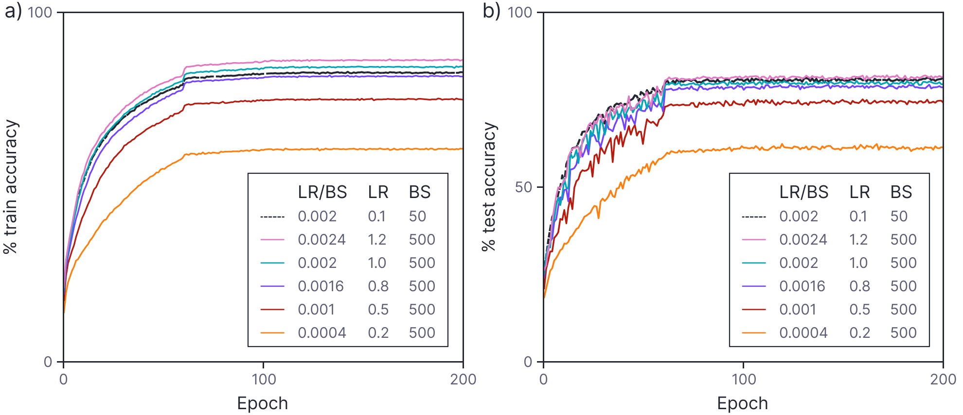
Figure 1.6 Learning rate to batch size ratio. a) Train accuracy of ResNet 56 on CIFAR-10 as a function of training epoch. Black dashed line indicates batch size of 50 and learning rate of 0.1. The remaining solid lines all have a batch size of 500, but different learning rates. The performance becomes more similar to the original line as the learning rate to batch size ratio becomes more similar. b) The same pattern is observed in the test dataset. Adapted from Jastrzebski et al. (2018)
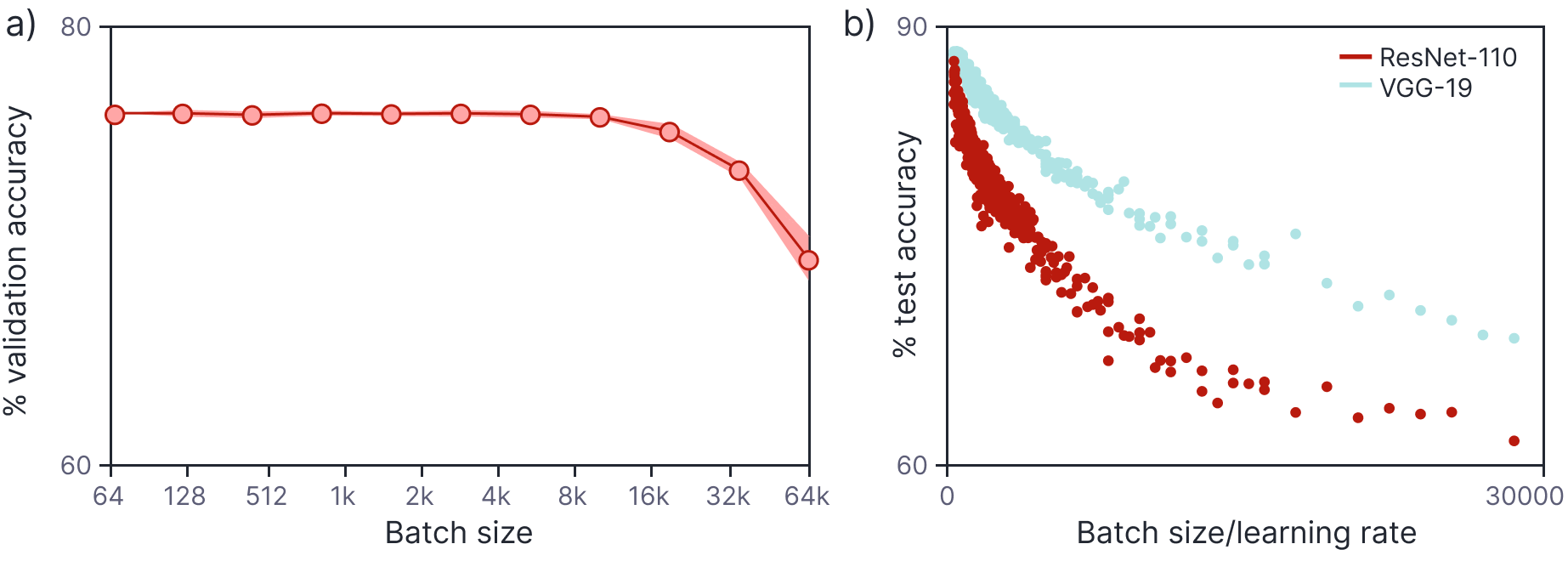
Figure 1.7 Learning rate to batch size ratio. a) ImageNet top-1 validation error vs. minibatch size, with the learning rate scaled linearly such that the ratio stays the same across all points. The accuracy stays the same over a wide range of batch sizes. Adapted from Goyal et al. (2017). b) Generalization of two models on the CIFAR-10 database depends on the ratio of batch size to the learning rate. As the batch size increases, generalization decreases. As the learning rate increases, generalization increases. Adapted from He et al. (2019).
This relation is only true for pure stochastic gradient descent. Malladi et al. (2022) derive SDE approximations for RMSProp and Adam and obtain a square root scaling rule; when we increase the batch size by a factor of $\kappa$, we should increase the learning rate by a factor of $\sqrt{\kappa}$ to maintain the same underlying SDE.
Implications for convergence
At convergence, the SGD algorithm will approach a minimum of the loss surface. For deep neural networks, the exact minimum will typically have zero loss (since neural networks can usually fit the training data exactly). However, the expected final loss of the SGD algorithm is not zero; the SGD algorithm will oscillate around the ideal zero loss position, and hence always have a finite loss (figure 1.8). We can relate (i) the shape of the minimum and (ii) the expected final loss to the stochastic gradient flow equation and see how these relate to the batch size and learning rate.
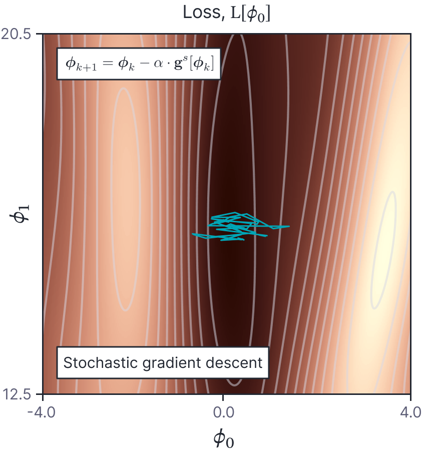
Figure 1.8 SGD at convergence. At convergence the SGD algorithm oscillates around the minimum point. The expected loss (average height of these points) can be related to the shape of the minimum using the stochastic gradient flow equation.
Consider approximating the minimum in the loss surface as a quadratic bowl with zero loss at the center and a shape described by the Hessian matrix $\mathbf{H}$. The covariance $\boldsymbol\Sigma$ of the gradients at convergence and the Hessian $\mathbf{H}$ describing the shape of the surface can be shown (non-obviously) to be approximately equal. A proof of this result is given at the end of the article.
Change of variables
We’ll now make a change of variables that allows us to find a closed-form solution to the stochastic differential equation around this minimum. We treat $\mathbf{H}\approx \boldsymbol\Sigma$ for this analysis and both are positive definite and so have eigen-decompositions $\mathbf{H} = \boldsymbol\Sigma = \mathbf{V}\boldsymbol\Lambda\mathbf{V}^{T}$ where $\mathbf{V}$ is an orthogonal matrix and $\boldsymbol\Lambda$ is a diagonal matrix. We make the change of variables $\boldsymbol\theta = \mathbf{V}^T(\boldsymbol\phi-\boldsymbol\phi^*)$ where $\boldsymbol\phi^{*}$ represents the parameters at the minimum. This moves to a coordinate system where the minimum is at the origin and the Hessian matrix is diagonal (figure 1.9).
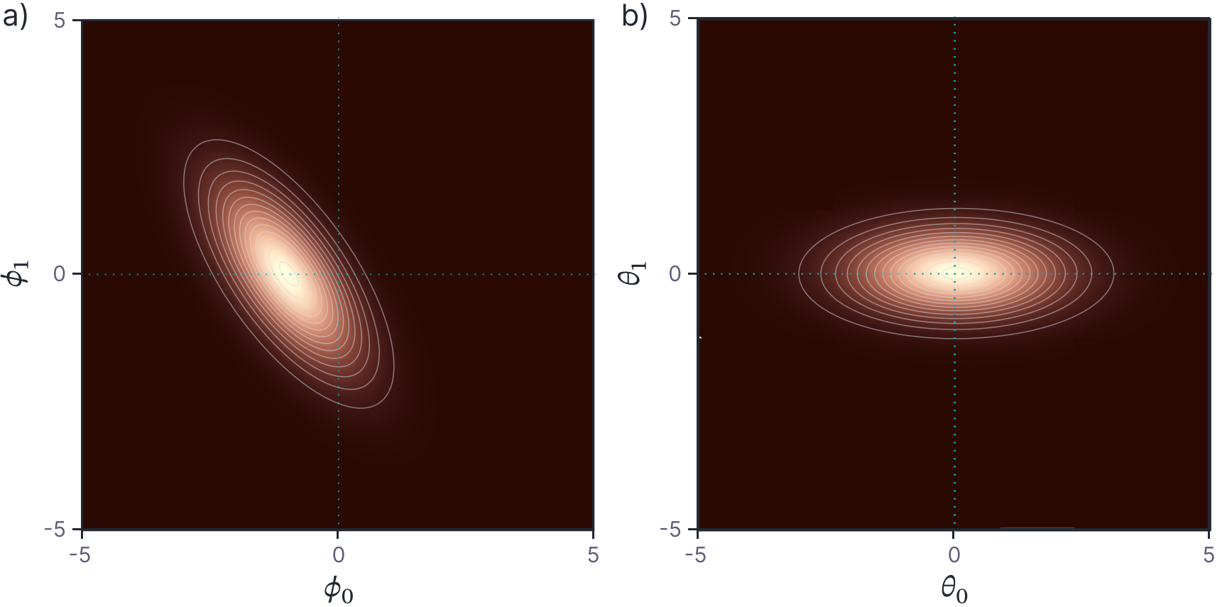
Figure 1.9 Change of variables. a) Loss function in original coordinate system is approximated by a quadratic bowl which is defined by the position of the minimum and the Hessian matrix of the quadratic (which defines the shape). b) We transform the loss function so that the minimum is at the origin and the isocontours of the quadratic bowl are aligned with the new axes.
To apply this change of variables to the stochastic gradient flow equation, we use the multivariate version of Itô’s lemma, which results in a new SDE:
\begin{equation}\label{eq:ode9_sde_after_ito2}
d\boldsymbol\theta[\boldsymbol\phi,t] = – \boldsymbol\Lambda \boldsymbol\theta dt + \sqrt{\frac{\alpha}{|\mathcal{B}|}}\boldsymbol\Lambda^{1/2}d\mathbf{w}.
\tag{1.20}
\end{equation}
See the end of the article for a proof of this result.
Trade-off between expected loss and width of minimum
Equation 1.49 is a multivariate version of the Ornstein-Uhlenbeck process, and as such it can be solved in closed form. In this case, it converges to a normal distribution with mean $\mathbb{E}[\boldsymbol\theta]=\mathbf{0}$ (as we expect, since the variable is defined as the deviation from the best parameters) and covariance matrix $\mathbb{E}[\boldsymbol\theta\boldsymbol\theta^{T}] = (\alpha/2|\mathcal{B}|)\mathbf{I}$.
The expectation $\mathbb{E}[L[\boldsymbol\theta]]$ of the loss $L$ in terms of the new parameters $\boldsymbol\theta$ can be written as:
\begin{eqnarray}
\mathbb{E}\Bigl[L[\boldsymbol\phi]\Bigr] &=& \mathbb{E}\left[\frac{1}{2}(\boldsymbol\phi-\boldsymbol\phi^{*})^T\mathbf{H}(\boldsymbol\phi-\boldsymbol\phi^{*})\right]\nonumber\\
&=& \mathbb{E}\left[\frac{1}{2}\boldsymbol\theta^{T}\mathbf{V}^T\mathbf{H}\mathbf{V}\boldsymbol\theta\right]\nonumber\\
&=& \mathbb{E}\left[\frac{1}{2}\boldsymbol\theta^{T}\mathbf{V}^T(\mathbf{V}\boldsymbol\Lambda\mathbf{V}^T)\mathbf{V}\boldsymbol\theta\right]\nonumber\\
&=& \mathbb{E}\left[\frac{1}{2}\boldsymbol\theta^{T}\boldsymbol\Lambda\boldsymbol\theta\right] \nonumber \\
&=& \frac{\alpha}{4|\mathcal{B}|}\operatorname{Tr}[\boldsymbol\Lambda] = \frac{\alpha}{4|\mathcal{B}|}\operatorname{Tr}[\mathbf{H}].
\tag{1.21}
\end{eqnarray}
This relation shows that there is a trade-off between the width of the minimum (captured by $\operatorname{Tr}[\mathbf{H}]$) and the expected loss $\mathbb{E}[L[\boldsymbol\phi]]$; as the minimum becomes wider ($\operatorname{Tr}[\mathbf{H}]$ decreases), the expected loss decreases. This trade-off is mediated by the learning rate to batch size ratio. For a fixed expected loss, a smaller batch size or a larger learning rate tends to yield better performance as it corresponds to a wider minimum that generalizes better.
Implicit regularization
In the previous sections, we derived the gradient flow and stochastic gradient flow equations. These describe gradient descent and stochastic gradient descent in the idealized situation of infinitesimal step sizes. In practice, however, we approximate this ideal situation by using a finite step size in the gradient descent and stochastic gradient descent algorithms.
In this section, we characterize the difference between the ideal case and the approximation. It transpires that neither gradient descent nor stochastic gradient descent moves neutrally to the minimum of the loss function; each exhibits a preference for some solutions over others. This is known as implicit regularization.
Implicit regularization in gradient descent
This deviation can be understood by deriving a modified loss term $\tilde{L}$ for the continuous case that arrives at the same place as the discretized version on the original loss $L$ (figure 1.10). We’ll now derive an expression for this modified loss term.
Recall that the gradient descent step is:
\begin{equation}\label{eq:reg_imp_discrete}
\boldsymbol\phi_{k+1} = \boldsymbol\phi_{k} – \alpha \cdot \textbf{g}[\boldsymbol\phi_k],
\tag{1.22}
\end{equation}
where $\textbf{g}[\boldsymbol\phi_k]$ is the gradient of the loss function, and $\alpha$ is the step size. As $\alpha\rightarrow 0$, the gradient descent process can be described by the gradient flow equation:
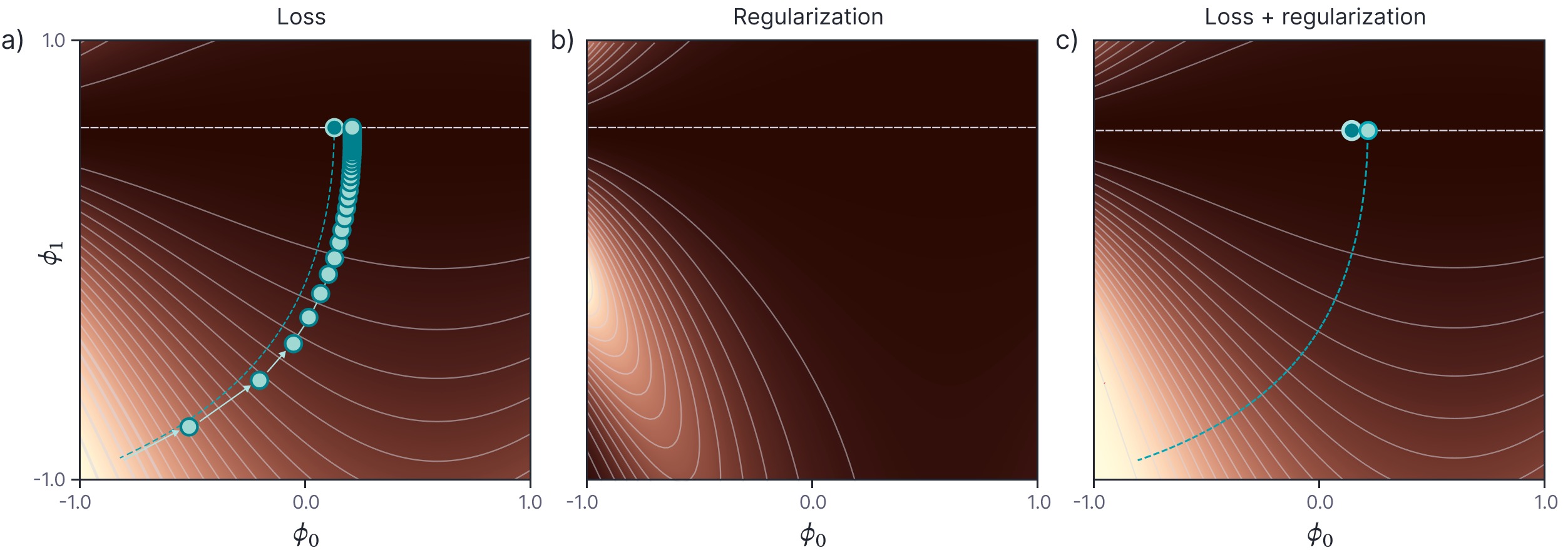
Figure 1.10 Implicit regularization in gradient descent. a) Loss function with family of global minima on horizontal line $\phi_{1}=0.61$. Dashed blue line shows continuous gradient descent path starting in bottom-left. Cyan trajectory shows discrete gradient descent with step size 0.1 (first few steps shown explicitly as arrows). The finite step size causes the paths to diverge and reach a different final position. b) This disparity can be approximated by adding a regularization term to the continuous gradient descent loss function that penalizes the squared gradient magnitude. c) After adding this term, the continuous gradient descent path converges to the same place that the discrete one did on the original function. Adapted from Prince (2023).
\begin{equation}
\frac{d\boldsymbol\phi}{dt} = -\textbf{g}[\boldsymbol\phi].
\tag{1.23}
\end{equation}
For typical step sizes $\alpha$, the discrete and continuous versions converge to different solutions. We can use backward error analysis to find a correction $\textbf{g}_{1}[\boldsymbol\phi]$ to the continuous version:
\begin{equation}\label{eq:reg_imp_correction}
\frac{d\boldsymbol\phi}{dt} \approx -\textbf{g}[\boldsymbol\phi] +\alpha \textbf{g}_{1}[\boldsymbol\phi],
\tag{1.24}
\end{equation}
so that it gives the same result as the discrete version.
Consider the first two terms of a Taylor expansion of the modified continuous solution $\boldsymbol\phi$ around initial position $\boldsymbol\phi_0$:
\begin{align}
\hspace{-1.5cm}\boldsymbol\phi[\alpha] \hspace{0.75cm}&\hspace{-0.75cm}\approx \left.\boldsymbol\phi \!+\! \alpha \frac{d\boldsymbol\phi}{dt} \!+\! \frac{\alpha^2}{2}\frac{d^2\boldsymbol\phi }{dt^2}\right|_{\boldsymbol\phi=\boldsymbol\phi_{0}}\nonumber \\
&\hspace{-0.75cm}\approx \left.\boldsymbol\phi \!+\! \alpha \left(-\textbf{g}[\boldsymbol\phi] \!+\!\alpha \textbf{g}_{1}[\boldsymbol\phi] \right) \!+\! \frac{\alpha^2}{2}\left(-\frac{\partial \textbf{g}[\boldsymbol\phi]}{\partial \boldsymbol\phi}\frac{d\boldsymbol\phi}{dt} \!+\!\alpha \frac{\partial \textbf{g}_{1}[\boldsymbol\phi]}{\partial \boldsymbol\phi}\frac{d\boldsymbol\phi}{dt}\right)\right|_{\boldsymbol\phi=\boldsymbol\phi_{0}}\nonumber \\
&\hspace{-0.75cm}= \left.\boldsymbol\phi \!+\! \alpha \left(-\textbf{g}[\boldsymbol\phi] \!+\!\alpha \textbf{g}_{1}[\boldsymbol\phi]\right) \!+\! \frac{\alpha^2}{2}\left(\frac{\partial \textbf{g}[\boldsymbol\phi]}{\partial \boldsymbol\phi}\textbf{g}[\boldsymbol\phi] -\alpha \frac{\partial \textbf{g}_{1}[\boldsymbol\phi]}{\partial \boldsymbol\phi}\textbf{g}[\boldsymbol\phi]\right)\right|_{\boldsymbol\phi=\boldsymbol\phi_{0}}\nonumber \\
&\hspace{-0.75cm}\approx \left.\boldsymbol\phi – \alpha \textbf{g}[\boldsymbol\phi] \!+\! \alpha^2\left(\textbf{g}_{1}[\boldsymbol\phi] \!+\!\frac{1}{2}\frac{\partial \textbf{g}[\boldsymbol\phi]}{\partial \boldsymbol\phi}\textbf{g}[\boldsymbol\phi]\right)\right|_{\boldsymbol\phi=\boldsymbol\phi_{0}},
\tag{1.25}
\end{align}
where in the second line, we have introduced the correction term $\frac{d\boldsymbol\phi}{dt} \approx -\textbf{g}[\boldsymbol\phi] +\alpha \textbf{g}_{1}[\boldsymbol\phi]$, and in the final line, we have removed terms of greater order than $\alpha^2$.
Note that the first two terms on the right-hand side $\boldsymbol\phi_0 + \alpha \textbf{g}[\boldsymbol\phi_0]$ are the same as the discrete update (equation 1.22). Hence, to make the continuous and discrete versions arrive at the same place, the third term on the right-hand side must equal zero, allowing us to solve for $\textbf{g}_{1}[\boldsymbol\phi]$:
\begin{equation}
\textbf{g}_{1}[\boldsymbol\phi] = -\frac{1}{2}\frac{\partial \textbf{g}[\boldsymbol\phi]}{\partial \boldsymbol\phi}\textbf{g}[\boldsymbol\phi].
\tag{1.26}
\end{equation}
It follows that during training the parameter update is approximately:
\begin{eqnarray}\label{eq:reg_imp_proof1}
\frac{d\boldsymbol\phi}{dt} &\approx& -\textbf{g}[\boldsymbol\phi] +\alpha \textbf{g}_{1}[\boldsymbol\phi] \nonumber \\
&=& -\frac{\partial L}{\partial \boldsymbol\phi}-\frac{\alpha}{2}\left(\frac{\partial^2 L}{\partial \boldsymbol\phi^2}\right)\frac{\partial L}{\partial \boldsymbol\phi}.
\tag{1.27}
\end{eqnarray}
This is equivalent to performing continuous gradient descent on the loss function:
\begin{equation}\label{eq:reg_imp_proof2}
L_{GD}[\boldsymbol\phi] = L[\boldsymbol\phi] + \frac{\alpha}{4} \left\lVert\frac{\partial L}{\partial \boldsymbol\phi} \right\rVert^{2},
\tag{1.28}
\end{equation}
because the right-hand side of equation 1.27 is the derivative of that in equation 1.31. In other words, the discrete trajectory is repelled from places where the gradient norm is large (the surface is steep). This does not change the position of the minima where the gradients are zero anyway. However, it changes the effective loss function elsewhere and modifies the optimization trajectory, which potentially converges to a different minimum. Implicit regularization due to gradient descent may be responsible for the observation that full batch gradient descent generalizes better with larger step sizes.
Implicit regularization in stochastic gradient descent
We can similarly consider how stochastic gradient descent deviates from stochastic gradient flow. Consider dividing the epoch into $B$ batches $\mathcal{B}_k$, each of equal size $|\mathcal{B}|$ so that $B = I / |\mathcal{B}|$. We can now rewrite the total loss $L[\boldsymbol\phi]$ as the sum of minibatch losses $L_k[\boldsymbol\phi]$:
\begin{equation}
L[\boldsymbol\phi] = \frac{1}{B} \sum_{j=1}^{B} L_{k}[\boldsymbol\phi],
\tag{1.29}
\end{equation}
where the minibatch loss is defined as:
\begin{equation}
L_{k}[\boldsymbol\phi]=\frac{1}{|\mathcal{B}|} \sum_{i\in\mathcal{B}_k} \ell_i.
\tag{1.30}
\end{equation}
After one epoch, the modified loss can be written as:
\begin{eqnarray}
L_{SGD}[\boldsymbol\phi] &=& L[\boldsymbol\phi] + \frac{\alpha}{4 B} \sum_{k=1}^{B}\left\lVert\frac{\partial L_k}{\partial \boldsymbol\phi} \right\rVert^{2}.
\tag{1.31}
\end{eqnarray}
We now manipulate this expression into a more interpretable form. We start by adding and subtracting a constant term:
\begin{align}\label{eq:ode9_implicit_sgd_proof}
\hspace{-1.5cm}L_{SGD}[\boldsymbol\phi] \hspace{0.75cm}&\hspace{-0.75cm}= L[\boldsymbol\phi] \!+\! \frac{\alpha}{2} \left\lVert\frac{\partial L}{\partial \boldsymbol\phi} \right\rVert^{2} – \frac{\alpha}{2} \left\lVert\frac{\partial L}{\partial \boldsymbol\phi} \right\rVert^{2}\!+\! \frac{\alpha}{4 B} \sum_{k=1}^{B}\left\lVert\frac{\partial L_k}{\partial \boldsymbol\phi} \right\rVert^{2}\nonumber \\
&\hspace{-0.75cm}= L[\boldsymbol\phi] \!+\! \frac{\alpha}{2} \left\lVert\frac{\partial L}{\partial \boldsymbol\phi} \right\rVert^{2} – \frac{\alpha}{2} \frac{\partial L}{\partial \boldsymbol\phi}^T\frac{\partial L}{\partial \boldsymbol\phi}\!+\! \frac{\alpha}{4 B} \sum_{k=1}^{B}\left\lVert\frac{\partial L_k}{\partial \boldsymbol\phi} \right\rVert^{2}\nonumber \\
&\hspace{-0.75cm}= L[\boldsymbol\phi] + \frac{\alpha}{2} \left\lVert\frac{\partial L}{\partial \boldsymbol\phi} \right\rVert^{2} – \frac{\alpha}{2B} \sum_{k=1}^{B}\frac{\partial L_k}{\partial \boldsymbol\phi}^T\frac{\partial L}{\partial \boldsymbol\phi}\!+\! \frac{\alpha}{4 B} \sum_{k=1}^{B}\left\lVert\frac{\partial L_k}{\partial \boldsymbol\phi} \right\rVert^{2}\nonumber \\
&\hspace{-0.75cm}= L[\boldsymbol\phi] \!+\! \frac{\alpha}{4} \left\lVert\frac{\partial L}{\partial \boldsymbol\phi} \right\rVert^{2} \!+\! \frac{\alpha}{4B}\sum_{k=1}^{B}\left(\left\lVert\frac{\partial L_k}{\partial \boldsymbol\phi} \right\rVert^{2} \!+\!\left\lVert\frac{\partial L}{\partial \boldsymbol\phi} \right\rVert^{2} – \frac{\partial L_k}{\partial \boldsymbol\phi}^T\frac{\partial L}{\partial \boldsymbol\phi}\right)\nonumber \\
&\hspace{-0.75cm}= L[\boldsymbol\phi] \!+\! \frac{\alpha}{4} \left\lVert\frac{\partial L}{\partial \boldsymbol\phi} \right\rVert^{2} \!+\!\frac{\alpha}{4 B} \sum_{k=1}^{B}\left\lVert\frac{\partial L_k}{\partial \boldsymbol\phi} – \frac{\partial L}{\partial \boldsymbol\phi} \right\rVert^{2}
\tag{1.32}
\end{align}
where we write the norm explicitly in line two, and substitute $L[\boldsymbol\phi] = \frac{1}{B} \sum_{j=1}^{B} L_{k}[\boldsymbol\phi]$ between lines two and three. In line four we collect together terms inside a single summation and in the final line, we gather these terms into a new norm.
Since the second term in equation 1.32 is just the implicit regulation term from gradient descent, we can write:
\begin{eqnarray}\label{eq:reg_imp_sgd}
L_{SGD}[\boldsymbol\phi] &=& L_{GD}[\boldsymbol\phi]+\frac{\alpha}{4 B}\sum_{k=1}^{B}\left\lVert\frac{\partial L_{k}}{\partial \boldsymbol\phi} – \frac{\partial L}{\partial \boldsymbol\phi} \right\rVert^{2}
\tag{1.33}
\end{eqnarray}
Equation 1.35 reveals an extra regularization term, which corresponds to the variance of the gradients of the batch losses $L_{k}$. In other words, SGD implicitly favors places where the gradients are stable (where all the batches agree on the slope). Once more, this modifies the trajectory of the optimization process (figure 1.11) but does not necessarily change the position of the global minimum; if the model is over-parameterized, then it may fit all the training data exactly, so each of these gradient terms will be zero at the global minimum.
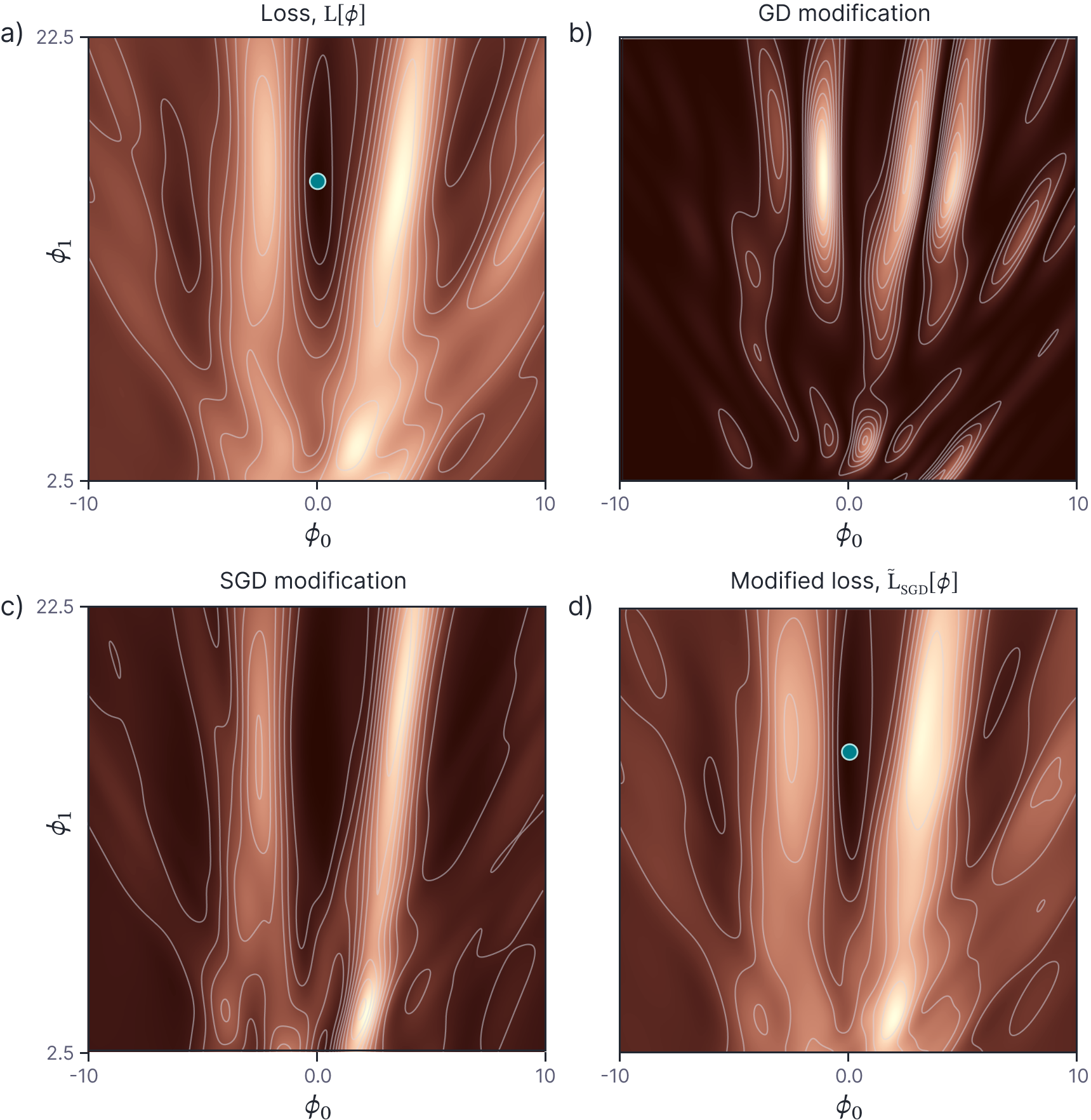
Figure 1.11 Implicit regularization for stochastic gradient descent. a) Original loss function. Blue point represents global minimum. b) Implicit regularization term from gradient descent penalizes the squared gradient magnitude. c) Additional implicit regularization from stochastic gradient descent penalizes the variance of the batch gradients. d) Modified loss function (sum of original loss plus two implicit regularization components). Blue point represents global minimum which may now be in a different place from panel (a). Adapted from Prince (2023).
We can make this equation more interpretable by noticing that the averaged norm is the trace of the batch covariance $\boldsymbol\Sigma_{\boldsymbol\epsilon}$ that we derived in equation 1.15:
\begin{equation}
\frac{1}{B}\sum_{k=1}^{B}\left\lVert\frac{\partial L_{k}}{\partial \boldsymbol\phi} – \frac{\partial L}{\partial \boldsymbol\phi} \right\rVert^{2} = \operatorname{Tr}\bigl[\boldsymbol\Sigma_{\boldsymbol\epsilon}\bigr]\approx \operatorname{Tr}\left[\frac{1}{|\mathcal{B}|}\boldsymbol\Sigma[\boldsymbol\phi]\right] = \frac{1}{|\mathcal{B}|}\operatorname{Tr}\bigl[\boldsymbol\Sigma[\boldsymbol\phi]\bigr],
\tag{1.34}
\end{equation}
\noindent where $\boldsymbol\Sigma[\boldsymbol\phi]$ is individual gradient covariance. We can hence rewrite equation 1.35 as:
\begin{eqnarray}
L_{SGD}[\boldsymbol\phi] &\approx& L_{GD}[\boldsymbol\phi]+\frac{\alpha}{4 |\mathcal{B}|}\operatorname{Tr}\bigr[\boldsymbol\Sigma[\boldsymbol\phi]\bigl].
\tag{1.35}
\end{eqnarray}
The learning rate to batch size ratio reappears in this formulation, and this explains why increasing the learning rate and decreasing the batch size both improve test performance (figure 1.1); both of these manipulations increase the amount of implicit regularization due to stochastic gradient descent.
Further reading
The formulation of implicit regularization described in this section was developed by Barrett and Dherin (2021) and extended to stochastic gradient descent by Smith et al. (2021). Smith et al. (2020) and others have shown that stochastic gradient descent with small or moderate batch sizes outperforms full batch gradient descent on the test set, and this may in part be due to implicit regularization.
Conclusion
This article derived equations for gradient flow and stochastic gradient flow; these are the ODE and SDE that correspond to gradient descent and stochastic gradient descent with infinitesimal learning rates. The stochastic gradient flow equation reveals a critical dependence on the learning rate to batch-size ratio which explains the empirical trade-off in performance as we vary these two quantities. Stochastic gradient flow also reveals a trade-off between the width of the minimum and the expected final loss, where the trade-off between these factors is mediated by the learning rate to batch-size ratio.
In the second part of this article, we considered how gradient descent with finite step size differs from the ideal of gradient flow. We saw that we can characterize this difference as a regularization term that penalizes the squared gradient magnitude. A similar analysis of stochastic gradient descent predicts a regularization term that penalizes the variance of batch gradients.
In the next article (Part X of this series), we will consider neural ODEs. These consider what happens to residual networks when the number of layers becomes infinite but the changes they make become infinitesimal.
Proof of equality of 𝐇 and 𝚺
Consider the mean of the gradients $\mathbf{g}_i[\boldsymbol\phi]=\partial\ell_i/\partial \phi$:
\begin{equation}
\mathbb{E}\Bigl[\textbf{g}_i[\boldsymbol\phi]\Bigr] = \textbf{g}[\boldsymbol\phi] = \frac{1}{I}\sum_{i=1}^{I} \textbf{g}_{i}[\boldsymbol\phi],
\tag{1.36}
\end{equation}
and the expectation of the gradient norm:
\begin{equation}
\mathbb{E}\Bigl[\textbf{g}_i[\boldsymbol\phi]^{T}\textbf{g}_i[\boldsymbol\phi]\Bigr] = \frac{1}{I}\sum_{i=1}^{I} \textbf{g}_{i}[\boldsymbol\phi]^{T}\textbf{g}_{i}[\boldsymbol\phi].
\tag{1.37}
\end{equation}
When we are close to the minimum, the squared norm of the full gradient becomes close to zero (the function is flat), but the expected squared norm of the individual gradients associated with each data point is not zero (each data example may still exert a gradient, even if these gradients cancel out in aggregate), so we have:
\begin{equation}
\textbf{g}[\boldsymbol\phi]^{T}\textbf{g}[\boldsymbol\phi]\ll \frac{1}{I}\sum_{i=1}^{I} \textbf{g}_{i}[\boldsymbol\phi]^{T}\textbf{g}_{i}[\boldsymbol\phi],
\tag{1.38}
\end{equation}
and the sample covariance matrix around the minimum converges to:
\begin{eqnarray}
\boldsymbol\Sigma &=& \mathbb{E}\Bigl[\textbf{g}_i[\boldsymbol\phi]\textbf{g}_i[\boldsymbol\phi]^T\Bigr] – \textbf{g}[\boldsymbol\phi]^T\textbf{g}[\boldsymbol\phi]\nonumber \\ &\approx &\mathbb{E}\Bigl[\textbf{g}_i[\boldsymbol\phi]\textbf{g}_i[\boldsymbol\phi]^T\Bigr]\nonumber \\
&=& \frac{1}{I}\sum_{i=1}^{I} \textbf{g}_{i}[\boldsymbol\phi]\textbf{g}_{i}[\boldsymbol\phi]^{T}.
\tag{1.39}
\end{eqnarray}
Now, we note that the gradients are the derivatives of the individual loss terms $\ell_{i}$ and that these loss terms are usually framed as the negative log likelihood $\ell_i = -\log\bigr[p(\mathbf{y}_i |\mathbf{x}_i, \boldsymbol\phi)\bigl]$, so the sample covariance matrix can be written as:
\begin{eqnarray}
\boldsymbol\Sigma = \frac{1}{I} \sum_{i=1}^{I} \frac{\partial \log[p(\mathbf{y}_i |\mathbf{x}_i, \boldsymbol\phi)]}{\partial \boldsymbol\phi}\frac{\partial \log[p(\mathbf{y}_i |\mathbf{x}_i, \boldsymbol\phi)]}{\partial \boldsymbol\phi}^{T}.
\tag{1.40}
\end{eqnarray}
The Hessian for the probabilistic model can be written as:
\begin{eqnarray}
\mathbf{H} &=& \frac{\partial^2 L[\boldsymbol\phi]}{\partial \boldsymbol\phi \partial \boldsymbol\phi^T} \\
&=& -\frac{1}{I}\sum_{i=1}^{I} \frac{\partial^2 \log[p(\mathbf{y}_i|\mathbf{x}_i,\boldsymbol\phi)]}{\partial \boldsymbol\phi \partial \boldsymbol\phi^T}\nonumber\\
&=& -\frac{1}{I}\sum_{i=1}^{I} \frac{\partial}{\partial\boldsymbol\phi^T}\left(\frac{1}{p(\mathbf{y}_i | \mathbf{x}_i, \boldsymbol\phi)} \frac{\partial p(\mathbf{y}_i | \mathbf{x}_i, \boldsymbol\phi)}{\partial \boldsymbol\phi}\right) \nonumber\\
&=& -\frac{1}{I}\sum_{i=1}^{I}\left( -\frac{1}{p(\mathbf{y}_i | \mathbf{x}_i, \boldsymbol\phi)^2} \frac{\partial p(\mathbf{y}_i | \mathbf{x}_i, \boldsymbol\phi)}{\partial \boldsymbol\phi}\frac{\partial p(\mathbf{y}_i | \mathbf{x}_i, \boldsymbol\phi)}{\partial \boldsymbol\phi^T} + \frac{1}{p(\mathbf{y}_i | \mathbf{x}_i, \boldsymbol\phi)} \frac{\partial^2 p(\mathbf{y}_i | \mathbf{x}_i, \boldsymbol\phi)}{\partial \boldsymbol\phi\partial\boldsymbol\phi^T} \right)\nonumber \\
&=& \frac{1}{I}\sum_{i=1}^{I}\left(\frac{\partial \log[p(\mathbf{y}_i |\mathbf{x}_i, \boldsymbol\phi)]}{\partial \boldsymbol\phi}\frac{\partial \log[p(\mathbf{y}_i |\mathbf{x}_i, \boldsymbol\phi)]}{\partial \boldsymbol\phi}^{T} – \frac{1}{p(\mathbf{y}_i |\mathbf{x}_i, \boldsymbol\phi)} \frac{\partial^2 p(\mathbf{y}_i |\mathbf{x}_i, \boldsymbol\phi)}{\partial \boldsymbol\phi \partial\boldsymbol\phi^{T}}\right),\nonumber
\tag{1.41}
\end{eqnarray}
where we have used the product rule between lines three and four and the definition of the derivative of a logarithm between lines four and five.
Now, we see that in the case where the model has been trained and the model’s conditional probability distribution $p(\mathbf{y} |\mathbf{x}, \boldsymbol\phi)$ coincides with the actual training data distribution $p(\mathbf{y} |\mathbf{x})$, the second term has an expectation of zero:
\begin{eqnarray}
\mathbb{E}_{p(\mathbf{y},\mathbf{x})}\left[\frac{1}{p(\mathbf{y}_i |\mathbf{x}_i, \boldsymbol\phi)} \frac{\partial^2 p(\mathbf{y}_i |\mathbf{x}_i, \boldsymbol\phi)}{\partial \boldsymbol\phi \partial\boldsymbol\phi^{T}}\right]
&=& \int \int p(\mathbf{x},\mathbf{y}) \frac{1}{p(\mathbf{y}_i |\mathbf{x}_i, \boldsymbol\phi)} \frac{\partial^2 p(\mathbf{y}_i |\mathbf{x}_i, \boldsymbol\phi)}{\partial \boldsymbol\phi \partial\boldsymbol\phi^{T}} d\mathbf{x}d\mathbf{y}\nonumber\\
&=& \int p(\mathbf{x}) \int \frac{p(\mathbf{y}|\mathbf{x})}{p(\mathbf{y}_i |\mathbf{x}_i, \boldsymbol\phi)} \frac{\partial^2 p(\mathbf{y}_i |\mathbf{x}_i, \boldsymbol\phi)}{\partial \boldsymbol\phi \partial\boldsymbol\phi^{T}} d\mathbf{x}d\mathbf{y}\nonumber\\
&\approx& \int p(\mathbf{x}) \int \frac{\partial^2 p(\mathbf{y}_i |\mathbf{x}_i, \boldsymbol\phi)}{\partial \boldsymbol\phi \partial\boldsymbol\phi^{T}} d\mathbf{x}d\mathbf{y}\nonumber\\
&=& \int p(\mathbf{x}) \frac{\partial^2 }{\partial \boldsymbol\phi \partial\boldsymbol\phi^{T}}\int p(\mathbf{y}_i |\mathbf{x}_i, \boldsymbol\phi)\, d\mathbf{y}\, d\mathbf{x}\nonumber\\ &=& \int p(\mathbf{x}) \frac{\partial^2 }{\partial \boldsymbol\phi \partial\boldsymbol\phi^{T}} 1 d\mathbf{x}\nonumber\\
&=& 0.
\tag{1.42}
\end{eqnarray}
It follows that the sample covariance $\boldsymbol\Sigma$ and the Hessian $\mathbf{H}$ are approximately the same:
\begin{equation}
\mathbf{H} \approx \frac{1}{I}\sum_{i=1}^{I}\frac{\partial \log[p(\mathbf{y}_i |\mathbf{x}_i, \boldsymbol\phi)]}{\partial \boldsymbol\phi}\frac{\partial \log[p(\mathbf{y}_i |\mathbf{x}_i, \boldsymbol\phi)]}{\partial \boldsymbol\phi}^{T} = \boldsymbol\Sigma.
\tag{1.43}
\end{equation}
Proof of change of variables
To change variables, we use the multivariate version of Itô’s lemma (see part VII of this series of articles):
\begin{equation}
\hspace{-1.0cm}d\boldsymbol\theta[\boldsymbol\phi,t] = \left(\frac{\partial \boldsymbol\theta}{\partial t} + \frac{\partial \boldsymbol\theta}{\partial \boldsymbol\phi}\textbf{m}[\boldsymbol\phi,t] + \frac{1}{2} \frac{\partial^{2} \boldsymbol\theta}{\partial \boldsymbol\phi\partial \boldsymbol\phi^{T}}\textbf{s}[\boldsymbol\phi,t]^{2} \right)dt + \frac{\partial \boldsymbol\theta}{\partial \boldsymbol\phi} \textbf{s}[\boldsymbol\phi,t]d\mathbf{w},
\tag{1.44}
\end{equation}
where in our case $\textbf{m}[\boldsymbol\phi,t]=-\textbf{g}[\boldsymbol\phi]$ and $\textbf{s}[\boldsymbol\phi,t] = \sqrt{\alpha/|\mathcal{B}|}\cdot \boldsymbol\Sigma^{1/2}[\boldsymbol\phi]$ are the drift and diffusion terms of the original SDE. In our case, $\partial \boldsymbol\theta/\partial t=0$, $\partial \boldsymbol\theta/\partial \boldsymbol\phi = \mathbf{V}^T$, and the second derivative term is zero giving:
\begin{equation}\label{eq:ode9_sde_after_ito}
d\boldsymbol\theta[\boldsymbol\phi,t] = -\mathbf{V}^T\textbf{g}[\boldsymbol\phi] dt + \mathbf{V}^{T} \sqrt{\frac{\alpha}{|\mathcal{B}|}}\cdot \boldsymbol\Sigma[\boldsymbol\phi]^{1/2}d\mathbf{w}.
\tag{1.45}
\end{equation}
We can manipulate both of these terms to simpler forms. For the first term, we note that the gradient $\textbf{g}[\boldsymbol\phi]=\partial L /\partial \boldsymbol\phi$ is approximately equal to $\frac{1}{2}\partial (\boldsymbol\phi-\boldsymbol\phi^*)^T\mathbf{H}(\boldsymbol\phi-\boldsymbol\phi^{*})/\partial \boldsymbol\phi$ = $\mathbf{H}(\boldsymbol\phi-\boldsymbol\phi^{*})$ in the vicinity of the minimum, giving:
\begin{eqnarray}
\mathbf{V}^T\textbf{g}[\boldsymbol\phi] dt &=& \mathbf{V}^{T}\mathbf{H}(\boldsymbol\phi-\boldsymbol\phi^{*})\nonumber \\
&=& \mathbf{V}^{T}\mathbf{V}\boldsymbol\Lambda\mathbf{V}^{T}(\boldsymbol\phi-\boldsymbol\phi^{*})\\
&=& \boldsymbol\Lambda \boldsymbol\theta,
\tag{1.46}
\end{eqnarray}
where we have used the fact that $\mathbf{V}^T\mathbf{V}=\mathbf{I}$ and substituted in the definition of $\boldsymbol\theta$ in the last line. For the second term, we have:
\begin{eqnarray} \mathbf{V}^{T} \sqrt{\frac{\alpha}{|\mathcal{B}|}}\boldsymbol\Sigma^{1/2}[\boldsymbol\phi]d\mathbf{w} &=&
\mathbf{V}^{T} \sqrt{\frac{\alpha}{|\mathcal{B}|}}\mathbf{V}\boldsymbol\Lambda^{1/2}d\mathbf{w}\nonumber\\
&=& \sqrt{\frac{\alpha}{|\mathcal{B}|}}\boldsymbol\Lambda^{1/2}d\mathbf{w}.
\tag{1.47}
\end{eqnarray}
Finally, substituting these results into equation 1.45, we get:
\begin{equation}
d\boldsymbol\theta[\boldsymbol\phi,t] = – \boldsymbol\Lambda \boldsymbol\theta dt + \sqrt{\frac{\alpha}{|\mathcal{B}|}}\boldsymbol\Lambda^{1/2}d\mathbf{w}.
\tag{1.48}
\end{equation}